Beginner friendly training and prediction with CNNs
Convolutional Neural Networks (CNNs) are a popular tool for developing automated machine learning classifiers on images or image-like samples. By converting audio into a two-dimensional frequency vs. time representation such as a spectrogram, we can generate image-like samples that can be used to train CNNs. This tutorial demonstrates the basic use of OpenSoundscape’s preprocessors and cnn modules for training CNNs and making predictions using CNNs.
Under the hood, OpenSoundscape uses Pytorch for machine learning tasks. By using the class opensoundscape.torch.models.cnn.CNN, you can train and predict with PyTorch’s powerful CNN architectures in just a few lines of code.
First, let’s import some utilities.
[1]:
# the cnn module provides classes for training/predicting with various types of CNNs
from opensoundscape import CNN

#other utilities and packages
import torch
import pandas as pd
from pathlib import Path
import numpy as np
import pandas as pd
import random
import subprocess

#set up plotting
from matplotlib import pyplot as plt
plt.rcParams['figure.figsize']=[15,5] #for large visuals
%config InlineBackend.figure_format = 'retina'
Set manual seeds for pytorch and python. These ensure the training results are reproducible. You probably don’t want to do this when you actually train your model, but it’s useful for debugging.
[2]:
torch.manual_seed(0)
random.seed(0)
np.random.seed(0)
Prepare audio data
Download labeled audio files
Training a machine learning model requires some pre-labeled data. These data, in the form of audio recordings or spectrograms, are labeled with whether or not they contain the sound of the species of interest. These data can be obtained from online databases such as Xeno-Canto.org, or by labeling one’s own ARU data using a program like Cornell’s Raven sound analysis software.
The Kitzes Lab has created a small labeled dataset of short clips of American Woodcock vocalizations. You have two options for obtaining the folder of data, called woodcock_labeled_data:
- Run the following cell to download this small dataset. These commands require you to have
tarinstalled on your computer, as they will download and unzip a compressed file in.tar.gzformat. - Download a
.zipversion of the files by clicking here. You will have to unzip this folder and place the unzipped folder in the same folder that this notebook is in.
Note: Once you have the data, you do not need to run this cell again.
[3]:
subprocess.run(['curl','https://drive.google.com/uc?export=download&id=1Ly2M--dKzpx331cfUFdVuiP96QKGJz_P','-L', '-o','woodcock_labeled_data.tar.gz']) # Download the data
subprocess.run(["tar","-xzf", "woodcock_labeled_data.tar.gz"]) # Unzip the downloaded tar.gz file
subprocess.run(["rm", "woodcock_labeled_data.tar.gz"]) # Remove the file after its contents are unzipped
  % Total    % Received % Xferd  Average Speed   Time    Time     Time  Current
                                 Dload  Upload   Total   Spent    Left  Speed
  0     0    0     0    0     0      0      0 --:--:--  0:00:04 --:--:--     0
100 9499k  100 9499k    0     0   669k      0  0:00:14  0:00:14 --:--:--  316k
[3]:
CompletedProcess(args=['rm', 'woodcock_labeled_data.tar.gz'], returncode=0)
Generate one-hot encoded labels
The folder contains 2s long audio clips taken from an autonomous recording unit. It also contains a file woodcock_labels.csv which contains the names of each file and its corresponding label information, created using a program called Specky.
[4]:
#load Specky output: a table of labeled audio files
specky_table = pd.read_csv(Path("woodcock_labeled_data/woodcock_labels.csv"))
specky_table.head()
[4]:
| filename | woodcock | sound_type | |
|---|---|---|---|
| 0 | d4c40b6066b489518f8da83af1ee4984.wav | present | song |
| 1 | e84a4b60a4f2d049d73162ee99a7ead8.wav | absent | na |
| 2 | 79678c979ebb880d5ed6d56f26ba69ff.wav | present | song |
| 3 | 49890077267b569e142440fa39b3041c.wav | present | song |
| 4 | 0c453a87185d8c7ce05c5c5ac5d525dc.wav | present | song |
This table must provide an accurate path to the files of interest. For this self-contained tutorial, we can use relative paths (starting with a dot and referring to files in the same folder), but you may want to use absolute paths for your training.
[5]:
#update the paths to the audio files
specky_table.filename = ['./woodcock_labeled_data/'+f for f in specky_table.filename]
specky_table.head()
[5]:
| filename | woodcock | sound_type | |
|---|---|---|---|
| 0 | ./woodcock_labeled_data/d4c40b6066b489518f8da8... | present | song |
| 1 | ./woodcock_labeled_data/e84a4b60a4f2d049d73162... | absent | na |
| 2 | ./woodcock_labeled_data/79678c979ebb880d5ed6d5... | present | song |
| 3 | ./woodcock_labeled_data/49890077267b569e142440... | present | song |
| 4 | ./woodcock_labeled_data/0c453a87185d8c7ce05c5c... | present | song |
We then modify these labels, replacing present with 1 and absent with zero. Ones and zeros are the way that presences and absences are represented in a machine learning model.
[6]:
# create a new dataframe with the filenames from the previous table as the index
labels = pd.DataFrame(index=specky_table['filename'])

#convert 'present' to 1 and 'absent' to 0
labels['woodcock']=[1 if l=='present' else 0 for l in specky_table['woodcock']]

#look at the first rows
labels.head(3)
[6]:
| woodcock | |
|---|---|
| filename | |
| ./woodcock_labeled_data/d4c40b6066b489518f8da83af1ee4984.wav | 1 |
| ./woodcock_labeled_data/e84a4b60a4f2d049d73162ee99a7ead8.wav | 0 |
| ./woodcock_labeled_data/79678c979ebb880d5ed6d56f26ba69ff.wav | 1 |
Split into training and validation sets
We use a utility from sklearn to randomly divide the labeled samples into two sets. The first set, train_df, will be used to train the CNN, while the second set, valid_df, will be used to test how well the model can predict the classes of samples that it was not trained with.
During the training process, the CNN will go through all of the samples once every “epoch” for several (sometimes hundreds of) epochs. Each epoch usually consists of a “learning” step and a “validation” step. In the learning step, the CNN iterates through all of the training samples while the computer program is modifying the weights of the convolutional neural network. In the validation step, the program performs prediction on all of the validation samples and prints out metrics to assess how well the classifier generalizes to unseen data.
Note: using the random_state argument with a fixed number means that the “random” split will be exactly the same each time we run it. This is useful for reproducible results, but to get a different split each time you would not use the random_state argument.
[7]:
from sklearn.model_selection import train_test_split
train_df,validation_df = train_test_split(labels,test_size=0.2,random_state=1)
Create and train a model
Now, we create a convolutional neural network model object, train it on the train_dataset with validation from validation_dataset
Set up a one-class CNN
The purpose of this model is to predict the presence or absence of a single species, so it has one class “woodcock”. Its also possible to train models to recognize multiple species - we call these “multi-class models” and each category of sounds it learns to recognize is a “class”.
The model object should be initialized with a list of class names that matches the class names in the training dataset. Here we’ll use the resnet18 architecture, a popular and powerful architecture that makes a good starting point. For more details on other CNN architectures, see the “Advanced CNN Training” tutorial.
[8]:
# Create model object
classes = train_df.columns #in this case, there's just one class: ["woodcock"]
model = CNN('resnet18',classes=classes,sample_duration=2.0)
CAVEAT: the default audio preprocessing in this class bandpasses spectrograms to 0-11025 Hz. If your audio has a sample rate of less than 22050 Hz, the preprocessing will raise an error because the spectrogram will not contain the expected frequencies. In this case you could change the parameters of the bandpass action, or simply disable the bandpass action:
model.preprocessor.pipeline.bandpass.bypass=True
Inspect training images
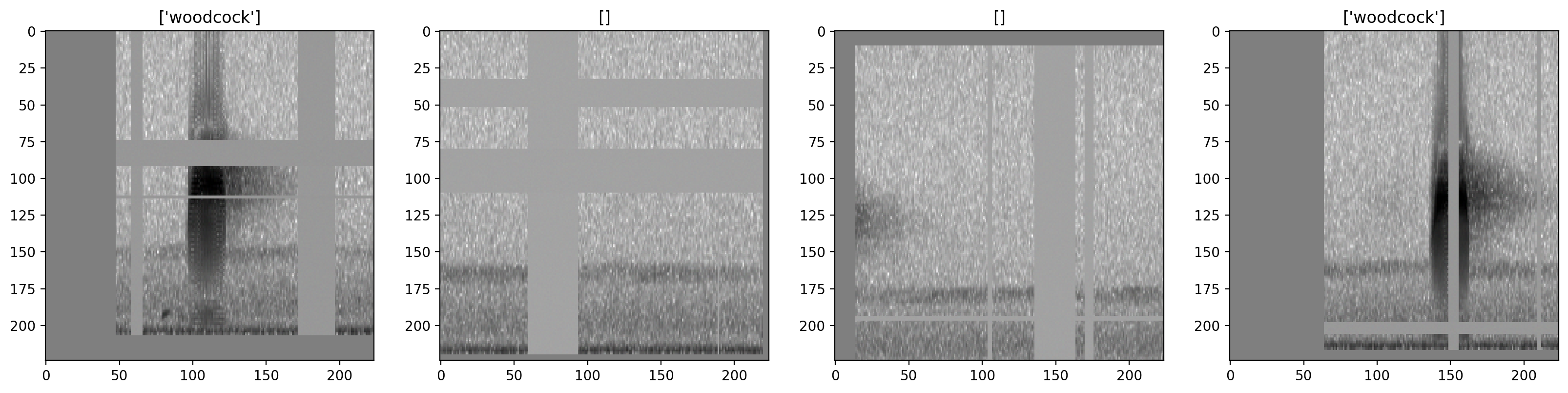
Before creating a machine learning algorithm, we strongly recommend making sure the images coming out of the preprocessor look like you expect them to. Here we generate images for a few samples.
[9]:
#helper functions to visualize processed samples
from opensoundscape.preprocess.utils import show_tensor_grid, show_tensor
from opensoundscape.ml.datasets import AudioFileDataset
Now, let’s check what the samples generated by our model look like
[10]:
#pick some random samples from the training set

sample_of_4 = train_df.sample(n=4)

#generate a dataset with the samples we wish to generate and the model's preprocessor
inspection_dataset = AudioFileDataset(sample_of_4, model.preprocessor)

#generate the samples using the dataset
samples = [sample.data for sample in inspection_dataset]
labels = [list(sample.labels[sample.labels>0].index) for sample in inspection_dataset]

#display the samples
_ = show_tensor_grid(samples,4,labels=labels)
/Users/SML161/miniconda3/envs/opso_dev/lib/python3.9/site-packages/matplotlib_inline/config.py:68: DeprecationWarning: InlineBackend._figure_format_changed is deprecated in traitlets 4.1: use @observe and @unobserve instead.
  def _figure_format_changed(self, name, old, new):
Clipping input data to the valid range for imshow with RGB data ([0..1] for floats or [0..255] for integers).
Clipping input data to the valid range for imshow with RGB data ([0..1] for floats or [0..255] for integers).
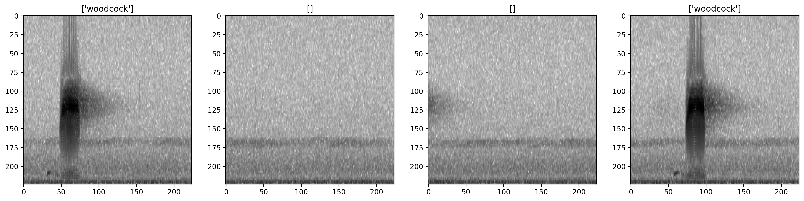
The dataset allows you to turn all augmentation off or on as desired. Inspect the unaugmented images as well:
[11]:
#turn augmentation off for the dataset
inspection_dataset.bypass_augmentations = True

#generate the samples without augmentation
samples = [sample.data for sample in inspection_dataset]
labels = [list(sample.labels[sample.labels>0].index) for sample in inspection_dataset]

#display the samples
_ = show_tensor_grid(samples,4,labels=labels)
Initilize Weights & Biases logging session
Weights and Biases (WandB) is a powerful and beautiful tool for logging and visualizing the machine learning model training process.
OpenSoundscape supports WandB integration, making it easy to visualize preprocessed samples and progress during training.
To use WandB, first create an account at https://wandb.ai/. The first time you use it on any computer, you’ll need to run wandb.login() either in the command line or in Python, and enter the API key from your settings page. The “Entity” or team option allows runs and projects to be shared across members in a group, making it easy to collaborate and see progress and results of other team members’ runs.
[12]:
try:
    import wandb
    wandb.login()
    wandb_session = wandb.init(
        entity='kitzeslab',
        project='opensoundscape_tutorials',
        name='cnn training tutorial'
    )
except:
    wandb_sesion = None
Failed to detect the name of this notebook, you can set it manually with the WANDB_NOTEBOOK_NAME environment variable to enable code saving.
wandb: Currently logged in as: samlapp (kitzeslab). Use `wandb login --relogin` to force relogin
/Users/SML161/opensoundscape/docs/tutorials/wandb/run-20230427_213711-rv67reaqTrain the model
Depending on the speed of your computer, training the CNN may take a few minutes.
We’ll only train for 5 epochs on this small dataset as a demonstration, but you’ll probably need to train for tens (or hundreds) of epochs on hundreds (or thousands) of training files to create a useful model.
Batch size refers to the number of samples that are simultaneously processed by the model. In practice, using larger batch sizes (64+) improves stability and generalizability of training, particularly for architectures (such as ResNet) that contain a ‘batch norm’ layer. Here we use a small batch size to keep the computational requirements for this tutorial low.
[13]:
model.train(
    train_df=train_df,
    validation_df=validation_df,
    save_path='./binary_train/', #where to save the trained model
    epochs=10,
    batch_size=8,
    save_interval=5, #save model every 5 epochs (the best model is always saved in addition)
    num_workers=0, #specify 4 if you have 4 CPU processes, eg; 0 means only the root process
    wandb_session=wandb_session
)


# let wandb know that we finished training successfully
wandb.unwatch(model.network)
wandb.finish()
wandb: logging graph, to disable use `wandb.watch(log_graph=False)`
Training Epoch 0
Epoch: 0 [batch 0/3, 0.00%]
        DistLoss: 0.694
Metrics:
Metrics:
        MAP: 0.637

Validation.
Metrics:
        MAP: 1.000

Training Epoch 1
Epoch: 1 [batch 0/3, 0.00%]
        DistLoss: 0.619
Metrics:
Metrics:
        MAP: 0.882

Validation.
Metrics:
        MAP: 1.000

Training Epoch 2
Epoch: 2 [batch 0/3, 0.00%]
        DistLoss: 0.749
Metrics:
Metrics:
        MAP: 0.862

Validation.
Metrics:
        MAP: 1.000

Training Epoch 3
Epoch: 3 [batch 0/3, 0.00%]
        DistLoss: 0.405
Metrics:
Metrics:
        MAP: 0.929

Validation.
Metrics:
        MAP: 1.000

Training Epoch 4
Epoch: 4 [batch 0/3, 0.00%]
        DistLoss: 0.279
Metrics:
Metrics:
        MAP: 0.945

Validation.
Metrics:
        MAP: 0.967

Training Epoch 5
Epoch: 5 [batch 0/3, 0.00%]
        DistLoss: 0.619
Metrics:
Metrics:
        MAP: 0.948

Validation.
Metrics:
        MAP: 0.967

Training Epoch 6
Epoch: 6 [batch 0/3, 0.00%]
        DistLoss: 0.672
Metrics:
Metrics:
        MAP: 0.955

Validation.
Metrics:
        MAP: 0.967

Training Epoch 7
Epoch: 7 [batch 0/3, 0.00%]
        DistLoss: 0.160
Metrics:
Metrics:
        MAP: 0.957

Validation.
Metrics:
        MAP: 0.927

Training Epoch 8
Epoch: 8 [batch 0/3, 0.00%]
        DistLoss: 0.427
Metrics:
Metrics:
        MAP: 0.956

Validation.
Metrics:
        MAP: 1.000

Training Epoch 9
Epoch: 9 [batch 0/3, 0.00%]
        DistLoss: 0.178
Metrics:
Metrics:
        MAP: 1.000

Validation.
Metrics:
        MAP: 1.000

Best Model Appears at Epoch 0 with Validation score 1.000.
Run history:
| epoch | ▁▂▃▃▄▅▆▆▇█ |
| loss | █▄▅▄▅▅▃▃▅▁ |
Run summary:
| epoch | 9 |
| loss | 0.1809 |
Synced 6 W&B file(s), 4 media file(s), 44 artifact file(s) and 0 other file(s)
./wandb/run-20230427_213711-rv67reaq/logsInspect metrics and samples using wandb
to see the wandb webpage generated by the original run of this notebook, visit https://wandb.ai/kitzeslab/opensoundscape_tutorials/runs/rv67reaq?workspace=user-samlapp
[14]:
wandb_session
[14]:
Visualize gradient activation maps
using gradient activation maps such as GradCAM, we can check what parts of the sample the model is paying attention to when it correctly (or incorrectly) labels a sample with a class.
Here, we can see that the American Woodcock vocalization in the sample is activating the network
[15]:
samples = model.generate_cams(samples=train_df.head(1))
samples[0].cam.plot()
Clipping input data to the valid range for imshow with RGB data ([0..1] for floats or [0..255] for integers).
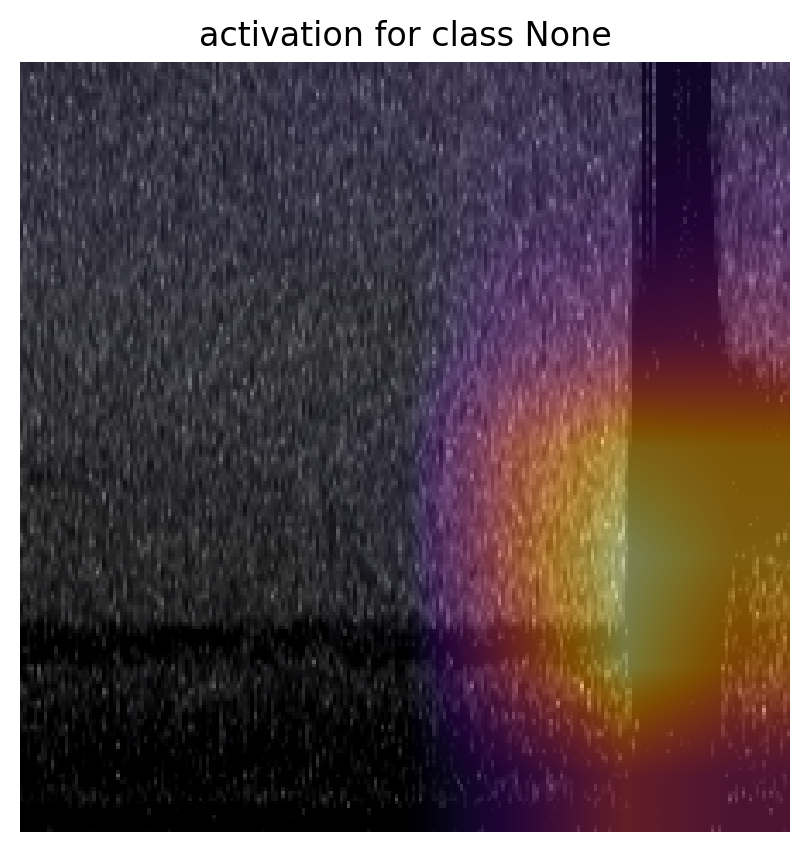
[15]:
(<Figure size 1500x500 with 1 Axes>,
 <AxesSubplot:title={'center':'activation for class None'}>)
You can also use generate_cams(...backprop=True) and cam.plot(...mode='backprop') or mode='backprop_and_activation' to see pixel-level activations of gradients. This will work best with a model trained more thoroughly than our toy model in this example.
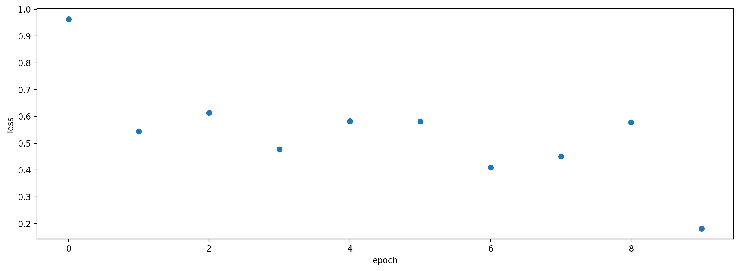
Plot the loss history
We can plot the loss from each epoch to check that our loss is declining. Loss should decline as the model learns, but may have ups and downs along the way.
[16]:
plt.scatter(model.loss_hist.keys(),model.loss_hist.values())
plt.xlabel('epoch')
plt.ylabel('loss')
[16]:
Text(0, 0.5, 'loss')
Printing and Logging outputs
We can log the outputs of the training process to a file, and/or print them. We can independently modify how much content is logged/printed with the model’s attributes model.verbose and model.logging_level. Content increases from level 0 (nothing) to 1 (standard), 2, 3, etc. For instance, let’s train for an epoch with lots of logged content but no printed output:
[17]:
model.logging_level = 3 #request lots of logged content
model.log_file = './binary_train/training_log.txt' #specify a file to log output to
Path(model.log_file).parent.mkdir(parents=True,exist_ok=True) #make the folder ./binary_train

model.verbose = 0 #don't print anything to the screen during training
model.train(
    train_df=train_df,
    validation_df=validation_df,
    save_path='./binary_train/', #where to save the trained model
    epochs=1,
    batch_size=8,
    save_interval=5, #save model every 5 epochs (the best model is always saved in addition)
    num_workers=0, #specify 4 if you have 4 CPU processes, eg; 0 means only the root process
)
Prediction
We haven’t actually trained a useful model in 5 epochs, but we can use the trained model to demonstrate how prediction works and show several of the settings useful for prediction.
We will run prediction on two one-minute clips of field data recorded by an AudioMoth acoustic recorded. The two files are located in woodcock_labeled_data/field_data
Predict on the field data
To run prediction, also known as “inference”, wich a CNN, we simply call model’s predict method and pass it a list of file paths (or a dataframe with file paths in the index).
The predict function will internally split audio files into the appropriate length clips for prediction and generate prediction scores for each clip.
- By default, there is no overlap between these clips, but we can specify a fraction of overlap with consecutive clips with the
overlap_fractionargument (eg, 0.5 for 50% overlap). - Additionally, if we want to predict on audio files that are already trimmed to the same duration as the training files, we can specify
split_files_into_clips=False.
Calling .predict() will return a dataframe with numeric (continuous score) predictions from the model for each sample and class (by default these are raw outputs from the model).
Let’s predict on the two field recordings:
[18]:
from glob import glob
field_recordings = glob('./woodcock_labeled_data/field_data/*')
field_recordings
[18]:
['./woodcock_labeled_data/field_data/60s_field_data_sample_1.wav',
 './woodcock_labeled_data/field_data/60s_field_data_sample_2.wav']
[19]:
prediction_scores_df = model.predict(field_recordings)
The predict function generated a dataframe with rows for each 2-second segment of each 1-minute audio clip. Let’s look at the first few rows:
[20]:
prediction_scores_df.head()
[20]:
| woodcock | |||
|---|---|---|---|
| file | start_time | end_time | |
| ./woodcock_labeled_data/field_data/60s_field_data_sample_1.wav | 0.0 | 2.0 | 1.785296 |
| 2.0 | 4.0 | 1.707386 | |
| 4.0 | 6.0 | 1.753464 | |
| 6.0 | 8.0 | 2.018827 | |
| 8.0 | 10.0 | 1.863675 |
Prediction can also be monitored with WandB by passing wandb_session to the wandb_session argument. This is especially useful for prediction runs that may take a long time.
Generate boolean predicted class labels (0/1) from the continuous scores
Note: Presence/absence predictions always have some error rates, sometimes large ones. It is not generally advisable to use these binary predictions as scientific observations without a thorough understanding of the model’s false-positive and false-negative rates.
There are two different ways we might want to predict class labels which reflect the nature of the classes themselves:
single target means that out of a set of classes, one and only one should be chosen for each sample. For instance, if our classes were days of the week, any single should be labeled with one and only one day of the week. In opensoundscape, use the function generate_single_target_labels() to convert scores to predicted single target labels. For each sample, the class with the highest score will recieve a label of 1 and all other classes will recieve a label of 0.
multi-target means that a sample can have 0, 1, or more than 1 labels. For instance, if our classes were the types of flowers in a photo, any given photo might have none of the classes, one class, or multiple different classes at once. In opensoundscape, use the function generate_multi_target_labels() to convert scores to predicted multi target labels. For each sample and each class, the class will be labeled 1 if its score is higher than a user-specified threshold and 0 otherwise. You
can choose to use a single threshold for all classes, or specify a different threshold for each class.
[21]:
from opensoundscape.metrics import predict_single_target_labels

score_df = model.predict(field_recordings)

pred_df = predict_single_target_labels(score_df)
pred_df.head()
[21]:
| woodcock | |||
|---|---|---|---|
| file | start_time | end_time | |
| ./woodcock_labeled_data/field_data/60s_field_data_sample_1.wav | 0.0 | 2.0 | 1 |
| 2.0 | 4.0 | 1 | |
| 4.0 | 6.0 | 1 | |
| 6.0 | 8.0 | 1 | |
| 8.0 | 10.0 | 1 |
The predict_multi_target_labels function allows you to select a threshold. If a score exceeds that threshold, the binary prediction is 1; otherwise, it is 0. You can also specify a list of thresholds, with one for each class
[22]:
from opensoundscape.metrics import predict_multi_target_labels

multi_target_pred_df = predict_multi_target_labels(score_df,threshold=0.99)
multi_target_pred_df.head()
[22]:
| woodcock | |||
|---|---|---|---|
| file | start_time | end_time | |
| ./woodcock_labeled_data/field_data/60s_field_data_sample_1.wav | 0.0 | 2.0 | 1 |
| 2.0 | 4.0 | 1 | |
| 4.0 | 6.0 | 1 | |
| 6.0 | 8.0 | 1 | |
| 8.0 | 10.0 | 1 |
Note that it is possible both the negative and positive classes are predicted to be present. This is because multi_target labeling assumes that the classes are not mutually exclusive. For a presence/absence model like the one above, single_target labeling is more appropriate.
Change the activation layer
We can modify the final activation layer to change the scores returned by the predict() function. Note that this does not impact the results of the binary predictions (described above), which are always calculated using a sigmoid transformation (for multi-target models) or softmax function (for single-target models).
Options include:
None: default. Just the raw outputs of the network, which are in (-inf, inf)'softmax': scores across all classes will sum to 1 for each sample'softmax_and_logit': softmax the scores across all classes so they sum to 1, then apply the “logit” transformation to these scores, taking them from [0,1] back to (-inf,inf)'sigmoid': transforms each score individually to [0, 1] without requiring that all scores sum to 1
In this case, since we are just looking at the output of one class, we can use the ‘sigmoid’ activation layer to put scores on the interval [0,1]
Let’s generate binary 0/1 predictions on the validation set. Since these samples are the same length as the training files, we’ll specify split_files_into_clips=False (we just want one prediction per file, we don’t want to divide each file into shorter clips).
[23]:
valid_scores = model.predict(
    validation_df,
    activation_layer='sigmoid',
    split_files_into_clips=False
)
Compare the softmax scores to the true labels for this dataset, side-by-side:
[24]:
valid_scores.columns = ['pred_woodcock']
validation_df.join(valid_scores).sample(5)
[24]:
| woodcock | pred_woodcock | |
|---|---|---|
| filename | ||
| ./woodcock_labeled_data/4afa902e823095e03ba23ebc398c35b7.wav | 1 | 0.989541 |
| ./woodcock_labeled_data/92647ab903049a9ee4125abdf7b24f2a.wav | 1 | 0.969963 |
| ./woodcock_labeled_data/75b2f63e032dbd6d197900495a16856f.wav | 1 | 0.957937 |
| ./woodcock_labeled_data/882de25226ed989b31274eead6630b47.wav | 1 | 0.999741 |
| ./woodcock_labeled_data/ad14ac7ffa729060712b442e55aebf0b.wav | 0 | 0.360559 |
We can directly compare our model’s confidence that woodcock is present with the original labels
Parallelizing prediction
Two parameters can be used to increase prediction efficiency, depending on the computational resources available:
num_workers: Pytorch’s method of parallelizing across cores (CPUs) - choose 0 to predict on the root process, or >1 if you want to use more than 1 CPU process.batch_size: number of samples to predict on simultaneously. You can try increasing this by factors of two until you get a memory error, which means your batch size is too large for your system.
[25]:
score_df = model.predict(
    validation_df,
    batch_size=8,
    num_workers=0,
)
Multi-class models
A multi-class model can have any number of classes, and can be either
- multi-target: any number of classes can be positive for one sample
- single-target: exactly one class is positive for each sample
Models that are multi-target benefit from a modified loss function, and we have implemented a special class that is specifically designed for multi-target problems called ResampleLoss. We can use it as follows:
[26]:
from opensoundscape.ml.cnn import use_resample_loss
model = CNN('resnet18',classes,2.0,single_target=False)
use_resample_loss(model)
print("model.single_target:", model.single_target)
model.single_target: False
Train
Training looks the same as in one-class models.
[27]:
model.train(
    train_df,
    validation_df,
    save_path='./multilabel_train/',
    epochs=1,
    batch_size=64,
    save_interval=100,
    num_workers=0,
)
Training Epoch 0
Epoch: 0 [batch 0/1, 0.00%]
        DistLoss: nan
Metrics:
Metrics:
        MAP: nan

Validation.
/Users/SML161/opensoundscape/opensoundscape/ml/cnn.py:700: UserWarning: Recieved empty list of predictions (or all nan)
  warnings.warn("Recieved empty list of predictions (or all nan)")
Best Model Appears at Epoch 0 with Validation score 0.000.
Note: since we used the same data as above, we just trained a 1 class model with “resample loss”. You should not actually use resample loss for single class models!
Predict
Prediction looks the same as demonstrated above, but make sure to think carefully:
- What
activation_layerdo you want? - If creating boolean (0/1 or True/False) predictions for each sample and class, is my model single-target (use
metrics.predict_single_target_labels) or multi-target (usemetrics.predict_multi_target_labels)?
For more detail on these choices, see the sections about activation layers and boolean predictions above.
Save and load models
Models can be easily saved to a file and loaded at a later time. If the model was saved with OpenSoundscape version >=0.6.1, the entire model object will be saved - including the class, cnn architecture, loss function, and training/validation datasets. Models saved with earlier versions of OpenSoundscape do not contain all of this information and may require that you know their class and architecture (see below).
Save and load a model
OpenSoundscape saves models automatically during training:
- The model saves a copy of itself
self.save_pathtoepoch-X.modelautomatically during training everysave_intervalepochs - The model keeps the file
best.modelupdated with the weights that achieve the best score on the validation dataset. By default the model is evaluated using the mean average precision (MAP) score, but you can overwritemodel.eval()if you want to use a different metric for the best model.
You can also save the model manually at any time with model.save(path)
[28]:
model1 = CNN('resnet18',classes,2.0,single_target=False)
# Save every 2 epochs
model1.train(
    train_df,
    validation_df,
    epochs=3,
    batch_size=8,
    save_path='./binary_train/',
    save_interval=2,
    num_workers=0
)
model1.save('./binary_train/my_favorite.model')
Training Epoch 0
Epoch: 0 [batch 0/3, 0.00%]
        DistLoss: 0.835
Metrics:
Metrics:
        MAP: 0.751

Validation.
Metrics:
        MAP: 1.000

Training Epoch 1
Epoch: 1 [batch 0/3, 0.00%]
        DistLoss: 0.411
Metrics:
Metrics:
        MAP: 0.819

Validation.
Metrics:
        MAP: 1.000

Training Epoch 2
Epoch: 2 [batch 0/3, 0.00%]
        DistLoss: 0.450
Metrics:
Metrics:
        MAP: 0.978

Validation.
Metrics:
        MAP: 1.000

Best Model Appears at Epoch 0 with Validation score 1.000.
Load
Re-load a saved model with the load_model function:
[29]:
from opensoundscape.ml.cnn import load_model
model = load_model('./binary_train/best.model')
Note on saving models and version compatability
Loading a model in a different version of OpenSoundscape than the version that saved the model may not work. To use a model across different versions of OpenSoundscape, you should save the model.network’s state dict using model.save_weights(path) as described in the “predicting with pre-trained models” tutorial. You can load weights from a saved state dict with model.load_weights(path). We recommend saving both the full model object (.save()) and the raw weights (.save_weights())
for models you plan to use in the future.
Models saved with OpenSoundscape 0.4.x and 0.5.x can be loaded with load_outdated_model - but be sure to update the model.preprocessor after loading to match the settings used during training. See the tutorial “predicting with pre-trained models” for more details on loading models from earlier OpenSoundscape versions.
Predict using saved (or pre-trained) model
Using a saved or downloaded model to run predictions on audio files is as simple as
- Loading a previously saved model
- Generating a list of files for prediction
- Running
model.predict()on the preprocessor
[30]:
# load the saved model
model = load_model('./binary_train/best.model')

#predict on a dataset
scores = model.predict(field_recordings, activation_layer='sigmoid')
NOTE: See the tutorial “predicting with pre-trained models” for loading and using models from earlier OpenSoundscape versions
Continue training from saved model
Similar to predicting using a saved model, we can also continue to train a model after loading it from a saved file.
Note that .load() loads the entire model object, which includes optimizer parameters and learning rate parameters from the saved model, in addition to the network weights.
[31]:
# Create architecture
model = load_model('./binary_train/best.model')

# Continue training from the checkpoint where the model was saved
model.train(train_df,validation_df,save_path='.',epochs=0)
Best Model Appears at Epoch 0 with Validation score 0.000.
Next steps
You now have seen the basic usage of training CNNs with OpenSoundscape and generating predictions.
Additional tutorials you might be interested in are: * Custom preprocessing: how to change spectrogram parameters, modify augmentation routines, etc. * Custom training: how to modify and customize model training * Predict with pre-trained CNNs: details on how to predict with pre-trained CNNs. Much of this information was covered in the tutorial above, but this tutorial also includes information about using models made with previous versions of OpenSoundscape
Finally, clean up and remove files created during this tutorial:
[32]:
import shutil
dirs = ['./multilabel_train', './binary_train', './woodcock_labeled_data']
for d in dirs:
    try:
        shutil.rmtree(d)
    except:
        pass
[ ]: