Audio

This tutorial demonstrates how to use OpenSoundscape to open, inspect, and modify audio files using the Audio class.

The class stores audio data (.samples: a 1d array containing the digital waveform signal) and metadata (.metadata, a dictionariy containing information such as sample rate, recording start time, etc). The .sample_rate attribute stores the audio sample rate in Hz.

The class’s methods give access to modifications such as trimming (.trim()), filtering (.bandpass(), .lowpass(), .highpass()) , resampling (.resample()), or extending (.loop(), .extend_to(), extend_by()) the signal. Properties provide measurements such as signal level (.dBFS, .rms) and duration (.duration).

Run this tutorial

This tutorial is more than a reference! It’s a Jupyter Notebook which you can run and modify on Google Colab or your own computer.

Link to tutorial	How to run tutorial
	The link opens the tutorial in Google Colab. Uncomment the “installation” line in the first cell to install OpenSoundscape.
	The link downloads the tutorial file to your computer. Follow the Jupyter installation instructions, then open the tutorial file in Jupyter.

# if this is a Google Colab notebook, install opensoundscape in the runtime environment
if 'google.colab' in str(get_ipython()):
  %pip install opensoundscape

# download a sample audio file
import requests
link = 'https://tinyurl.com/birds60s'
r = requests.get(link, allow_redirects=True)
with open('1min_audio.wav', 'wb') as f:
    f.write(r.content)

Import the Audio class from OpenSoundscape.

For more information about Python imports, review this article.

# Import Audio class from OpenSoundscape
from opensoundscape import Audio, audio

/Users/SML161/opensoundscape/opensoundscape/ml/cnn.py:18: TqdmExperimentalWarning: Using `tqdm.autonotebook.tqdm` in notebook mode. Use `tqdm.tqdm` instead to force console mode (e.g. in jupyter console)
  from tqdm.autonotebook import tqdm

Load audio files

The Audio class can load local files with .from_file() and online audio files with .from_url(). All common audio formats are supported (via the underlying SoundFile package).

Saving files is as simple as calling the .save() method, and again all common audio formats are supported.

Note: Loading some formats including .mp3 may require that you install FFmpeg first. FFmpeg comes pre-installed on many machines including on Google Colab. Note that .mp3 files cause some operations to slow down (e.g. loading a segment from a long file).

Here we download an example birdsong soundscape recorded by an AudioMoth autonomous recorder in Pennsylvania, USA.

# load an audio file from a file
# can be any file path to an audio file on your computer
path = './1min_audio.wav'
audio_object = Audio.from_file(path)

# returning the audio object from a cell will display a player widget
audio_object

This interactive playback widget is displayed when an Audio object is returned from a notebook cell. We can also create the widget with .show_widget():

# Create playback widget with normalized playback level
audio_object.show_widget(normalize=True)

Save audio files

save an audio object to a file:

audio_object.save('./my_audio.wav')

Load audio from a real-world time from AudioMoth recordings

OpenSoundscape parses metadata of files recorded on AudioMoth recorders, and can use the metadata to extract pieces of audio corresponding to specific real-world times. (Note that AudioMoth internal clocks can drift an estimated 10-60 seconds per month).

from datetime import datetime; import pytz

#this AudioMoth recording starts at 10:25:00 am on April 4th, 2020
file = './1min_audio.wav'

# define a time at which we want to extract an audio clip from an AudioMoth recording
# (15 seconds after the start of the recording)
start_time = pytz.timezone('UTC').localize(datetime(2020,4,4,10,25,15))

audio_length = 5 #seconds

# Load the entire audio file and print the start time and duration
a = Audio.from_file(file)
print(f"Entire audio file starts at {a.metadata['recording_start_time']} and has duration {a.duration}.")

# Load a segment of the audio file starting at the desired date and time
a = Audio.from_file(file, start_timestamp=start_time, duration=audio_length)
print(f"Loaded audio segment starts at {a.metadata['recording_start_time']} and has duration {a.duration}.")

Entire audio file starts at 2020-04-04 10:25:00+00:00 and has duration 60.0.
Loaded audio segment starts at 2020-04-04 10:25:15+00:00 and has duration 5.0.

Audio properties

Once an Audio object is loaded, you can inspect its attributes, including: * ``samples``: The actual digitized audio data * ``sample_rate``: The number of audio samples taken per second, required to understand the samples * ``metadata``: A dictionary of audio file metadata such as start time, recording device, and bit depth * ``duration``: The length of the recording, calculated by dividing the number of samples by the sample rate * ``rms`` (root mean square): The average amplitude of the digitized sound wave * ``dBFS`` (decibels relative to full scale): A general measure of “loudness” of a recording. Decibels are measured on a scale less than 0, with values closer to 0 being louder. An decrease in 6 decibels is equivalent to the sound being twice as far away.

print(f"First few samples: {audio_object.samples[:3]} ... ")
print(f"Number of samples: {len(audio_object.samples)}")
print(f"Sample rate: {audio_object.sample_rate} Hz")
print(f"Duration: {audio_object.duration} seconds")
print(f"RMS: {audio_object.rms:0.3f}")
print(f"dBFS: {audio_object.dBFS:0.1f}")

First few samples: [-0.00888062 -0.00344849  0.00378418] ...
Number of samples: 1920000
Sample rate: 32000 Hz
Duration: 60.0 seconds
RMS: 0.013
dBFS: -34.5

Metadata is parsed from the audio file’s header. Metadata from AudioMoth recordings’s “comment” field is parsed into extra information such as start time, battery state, and gain setting. Changes to the .metadata attribute of the Audio object are saved when an audio object is saved to a file.

audio_object.metadata

{'artist': 'AudioMoth 24526B065D325963',
 'comment': 'Recorded at 10:25:00 04/04/2020 (UTC) by AudioMoth 24526B065D325963 at gain setting 2 while battery state was 4.7V.',
 'samplerate': 32000,
 'format': 'WAV',
 'frames': 1920000,
 'sections': 1,
 'subtype': 'PCM_16',
 'recording_start_time': datetime.datetime(2020, 4, 4, 10, 25, tzinfo=datetime.timezone(datetime.timedelta(0), 'UTC')),
 'gain_setting': 2,
 'battery_state': 4.7,
 'device_id': 'AudioMoth 24526B065D325963',
 'channels': 1,
 'duration': 60.0}

Load a segment of a file

We can directly load a section of a .wav file very efficiently (even if the audio file is large) using the offset and duration parameters of Audio.from_file()

For example, let’s load 1 second of audio starting 2.0 seconds into the file:

audio_segment = Audio.from_file(
    file,
    offset=30.0,
    duration=1.0)
audio_segment.duration
audio_segment.show_widget()

Resample audio during load

By default, an audio object is loaded with the same sample rate as the source recording.

The sample_rate parameter of Audio.from_file allows you to re-sample the file during the creation of the object. This is useful when working with multiple files to ensure that all files have a consistent sampling rate.

Let’s load the same audio file as above, but specify a sampling rate of 22050 Hz.

audio_object_resample = Audio.from_file(file, sample_rate=22050)
audio_object_resample.sample_rate

22050

Load an audio file from a download link / URL

Note that this currently does not support retaining metadata

# load a Wood Thrush recording from Xeno Canto
url = 'https://xeno-canto.org/818024/download'
xc = Audio.from_url(url)
xc

Load multi-channel audio

The Audio class currently only supports single-channel (eg, not 2 chanel stereo). By default, multi-channel audio files are summed to mono (1 channel) when loading with Audio.from_file(). If you want to use separate audio channels, you can load a file into one Audio object per channel:

# since this file is only one channel, we get back a list with one Audio object
audio.load_channels_as_audio('./1min_audio.wav')

[<Audio(samples=(1920000,), sample_rate=32000)>]

Measure and analyze audio signals

Generate a frequency spectrum

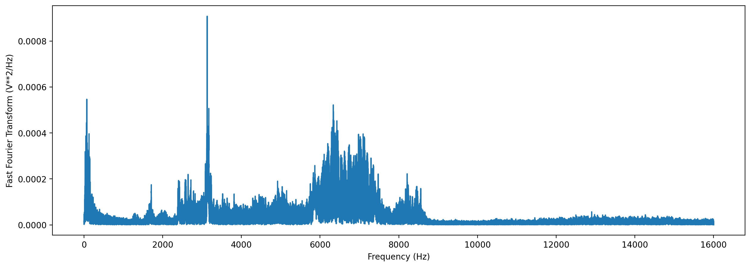
The .spectrum() method provides an easy way to compute a Fourier Transform on an audio object to measure its frequency composition.

# Calculate the fft
fft_spectrum, frequencies = audio_object.trim(0,5).spectrum()

# Plot settings
from matplotlib import pyplot as plt
plt.rcParams['figure.figsize']=[15,5] #for big visuals
%config InlineBackend.figure_format = 'retina'

# Plot
plt.plot(frequencies,fft_spectrum)
plt.ylabel('Fast Fourier Transform (V**2/Hz)')
plt.xlabel('Frequency (Hz)')
plt.show()

/Users/SML161/miniconda3/envs/opso_dev/lib/python3.9/site-packages/matplotlib_inline/config.py:68: DeprecationWarning: InlineBackend._figure_format_changed is deprecated in traitlets 4.1: use @observe and @unobserve instead.
  def _figure_format_changed(self, name, old, new):

Modify audio

The Audio class gives access to a variety of tools to change audio files, load them with special properties, or get information about them. Various examples are shown below.

For a description of the entire Audio object API, see the API documentation.

NOTE: Out-of-place operations

Functions that modify Audio (and Spectrogram) objects are “out of place”, meaning that they return a new, modified instance of Audio instead of modifying the original instance. This means that running a line

audio_object.resample(22050) # WRONG!

will not change the sample rate of audio_object! If your goal was to overwrite audio_object with the new, resampled audio, you would instead write

audio_object = audio_object.resample(22050)

Trim, extend, and loop audio

The .trim() method extracts audio from a specified time period in seconds (relative to the start of the audio object).

trimmed = audio_object.trim(0,5)
trimmed.duration

5.0

Extend audio object with silence to a target duration or by a specific ammount:

trimmed.extend_by(1).duration # extend by 1 second

6.0

trimmed.extend_to(10).duration # provide target duration in seconds

10.0

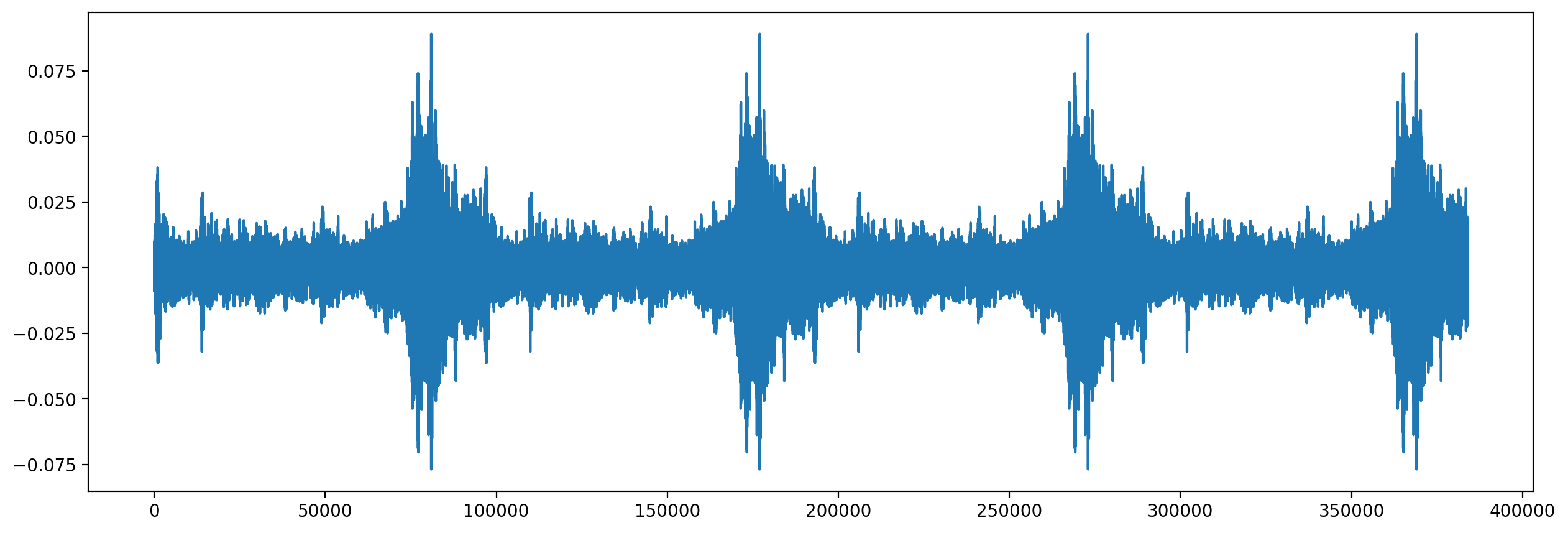
The .loop() method extends an audio file to a desired length (or number of repetitions) by looping the audio. Let’s loop the first 3 seconds of our audio object 4 times:

import warnings
warnings.filterwarnings("ignore")
import matplotlib.pyplot as plt
%config InlineBackend.figure_format = 'retina'

looped = audio_object.trim(0,3).loop(n=4)
print("Samples of looped clip:")
plt.plot(looped.samples)
plt.show()

Samples of looped clip:

Change the signal level (volume)

We can change the signal level by a specific amount, or normalize the signal

# make a quieter version of the audio, by reducing the gain by 10 dB
trimmed.apply_gain(-10)

# normalize the audio to -3 dBFS maximum amplitude
trimmed.normalize(peak_dBFS=-3)

print(f"max value before normalization: {trimmed.samples.max()}")

print(f"max value after normalization to full scale: {trimmed.normalize().samples.max()}")

max value before normalization: 0.234649658203125
max value after normalization to full scale: 1.0

Resample audio

The .resample() method resamples the audio object to a new sampling rate. This can be lower or higher than the original sampling rate.

Keep in mind that resampling can also be done while loading the file by specifying the desired sample rate in Audio.from_file

print(f"original sample rate: {audio_object.sample_rate}")
resampled = trimmed.resample(sample_rate=48000)
print(f"new sample rate: {resampled.sample_rate}")

original sample rate: 32000
new sample rate: 48000

Note that resampling audio to a lower rate reduces the sound frequencies that can be captured in the audio. The highest frequency that an audio file can capture is half of the sampling rate.

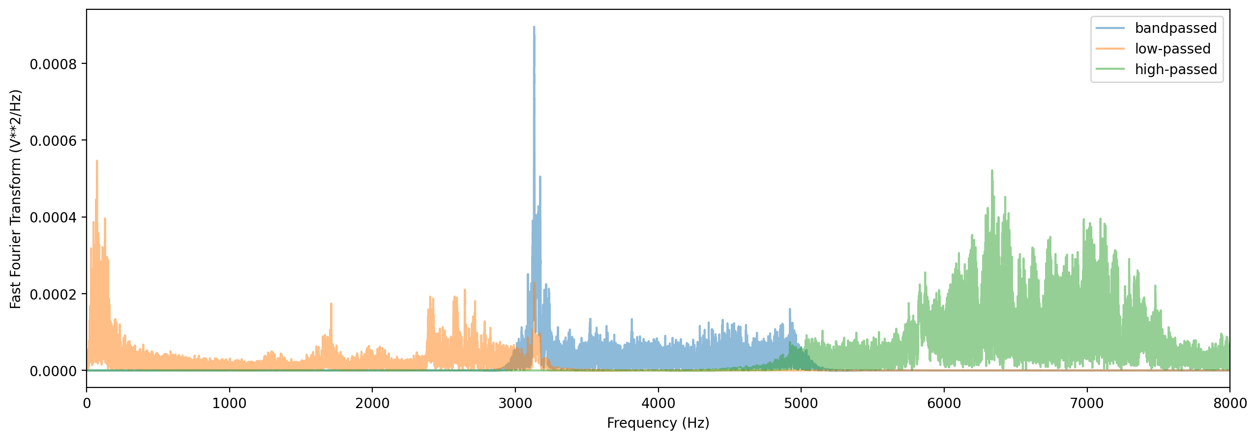
Filtering: low pass, high pass, bandpass

# Bandpass the audio file to limit its frequency range to 3000 Hz to 5000 Hz.
# The bandpass operation uses a Butterworth filter with a user-provided order.
bandpassed = trimmed.bandpass(low_f=3000,high_f=5000,order=12)

# Compute and plot spectrum
fft_spectrum, frequencies = bandpassed.spectrum()
plt.plot(frequencies,fft_spectrum,label='bandpassed',alpha=0.5)


# Low-pass the audio to remove frequencies above 3000 Hz
lowpassed = trimmed.lowpass(3000,order=12)
fft_spectrum, frequencies = lowpassed.spectrum()
plt.plot(frequencies,fft_spectrum,label='low-passed',alpha=0.5)

# High-pass the audio to remove frequencies below 5000 Hz
highpassed = trimmed.highpass(5000,order=12)
fft_spectrum, frequencies = highpassed.spectrum()
plt.plot(frequencies,fft_spectrum,label='high-passed',alpha=0.5)



# Plot settings
plt.ylabel('Fast Fourier Transform (V**2/Hz)')
plt.xlabel('Frequency (Hz)')
plt.xlim(0,8000)
plt.legend()
plt.show()

Split Audio into clips

The .split() method divides audio into even-lengthed clips, optionally with overlap between adjacent clips (default is no overlap). See the function’s documentation for options on how to handle the last clip.

The function returns a list containing Audio objects for each clip and a DataFrame giving the start and end times of each clip with respect to the original file.

Split without overlap

Split the audio into non-overlapping (mutually exclusive) clips

# Split into 5-second clips with no overlap between adjacent clips
clips, clip_df = audio_object.split(clip_duration=5,clip_overlap=0,final_clip=None)

# Check the duration of the Audio object in the first returned element
print(f"duration of first clip: {clips[0].duration}")

print(f"head of clip_df")
clip_df.head(3)

duration of first clip: 5.0
head of clip_df

	start_time	end_time
0	0.0	5.0
1	5.0	10.0
2	10.0	15.0

Split with overlap

Split the audio into overlapping clips.

Note that a negative “overlap” value would leave gaps between consecutive clips.

_, clip_df = audio_object.split(clip_duration=5,clip_overlap=2.5,final_clip=None)
print(f"head of clip_df")
clip_df.head()

head of clip_df

	start_time	end_time
0	0.0	5.0
1	2.5	7.5
2	5.0	10.0
3	7.5	12.5
4	10.0	15.0

Split and save

The Audio.split_and_save() method splits audio into clips and immediately saves them to files in a specified location.

You provide it with a naming prefix, and it will add on a suffix indicating the start and end times of the clip (eg _5.0-10.0s.wav). It returns just a DataFrame with the paths and start/end times for each clip (it does not return Audio objects).

The splitting options are the same as .split(): clip_duration, clip_overlap, and final_clip.

NOTE: If you want to split clips for use as a machine learning training dataset, you do not need to pre-split clips. See the machine learning tutorials for more information.

# Split into 5-second clips with no overlap between adjacent clips
from pathlib import Path
Path('./temp_audio').mkdir(exist_ok=True)
clip_df = audio_object.split_and_save(
    destination='./temp_audio',
    prefix='audio_clip_',
    clip_duration=5,
    clip_overlap=0,
    final_clip=None
)

print(f"head of clip_df")
clip_df.head()

head of clip_df

	start_time	end_time
file
./temp_audio/audio_clip__0.0s_5.0s.wav	0.0	5.0
./temp_audio/audio_clip__5.0s_10.0s.wav	5.0	10.0
./temp_audio/audio_clip__10.0s_15.0s.wav	10.0	15.0
./temp_audio/audio_clip__15.0s_20.0s.wav	15.0	20.0
./temp_audio/audio_clip__20.0s_25.0s.wav	20.0	25.0

The folder temp_audio should now contain 12 5-second clips created from the 60-second audio file.

Clean up: delete temp folder of saved audio clips

from shutil import rmtree
rmtree('./temp_audio')

Split and save “dry run”

we can use the dry_run=True option to produce only the clip_df but not actually process the audio. this is useful as a quick test to see if the function is behaving as expected, before doing any (potentially slow) splitting on huge audio files.

Just for fun, we’ll use an overlap of -5 in this example (5 second gap between each consecutive clip)

This function returns a DataFrame of clips, but does not actually process the audio files or write any new files.

clip_df = audio_object.split_and_save(
    destination='./temp_audio',
    prefix='audio_clip_',
    clip_duration=5,
    clip_overlap=-5,
    final_clip=None,
    dry_run=True,
)
clip_df

	start_time	end_time
file
./temp_audio/audio_clip__0.0s_5.0s.wav	0.0	5.0
./temp_audio/audio_clip__10.0s_15.0s.wav	10.0	15.0
./temp_audio/audio_clip__20.0s_25.0s.wav	20.0	25.0
./temp_audio/audio_clip__30.0s_35.0s.wav	30.0	35.0
./temp_audio/audio_clip__40.0s_45.0s.wav	40.0	45.0
./temp_audio/audio_clip__50.0s_55.0s.wav	50.0	55.0

Join and mix Audio objects

audio.concat() joins Audio objects end-to-end

audio.concat([audio_object, audio_object])

audio.mix() blends audio objects using a weighted sum

note that several parameters like gain, offsets, and duration allow you to manipulate how the Audio objects are mixed

# generate silence (audio waveform of all 0's)
audio.mix([audio_object, xc],duration=10, gain=[0,-6])

Generating noise and silence

Audio.silence(duration=5, sample_rate=22050) #generate silent clip (all 0s)

Audio.noise(color='pink', duration=5, sample_rate=22050) #generate pink noise

Clean up: run the following cell to delete the audio files saved during this tutorial

for path in ['./my_audio.wav', './1min_audio.wav']:
    try:
        Path(path).unlink()
    except:
        pass