Beginner friendly training and prediction with CNNs

Convolutional Neural Networks (CNNs) are a popular tool for developing automated machine learning classifiers on images or image-like samples. By converting audio into a two-dimensional frequency vs. time representation such as a spectrogram, we can generate image-like samples that can be used to train CNNs. This tutorial demonstrates the basic use of OpenSoundscape’s preprocessors and cnn modules for training CNNs and making predictions using CNNs.

Under the hood, OpenSoundscape uses Pytorch for machine learning tasks. By using OpenSoundscape’s CNN classes such as PytorchModel in combination with preprocessor classes such as CnnPreprocessor, you can train and predict with PyTorch’s powerful CNN architectures in just a few lines of code.

First, let’s import some utilities.

# Preprocessor classes are used to load, transform, and augment audio samples for use in a machine learing model
from opensoundscape.preprocess.preprocessors import CnnPreprocessor

# the cnn module provides classes for training/predicting with various types of CNNs
from opensoundscape.torch.models.cnn import PytorchModel

#other utilities and packages
import torch
import pandas as pd
from pathlib import Path
import numpy as np
import pandas as pd
import random
import subprocess

#set up plotting
from matplotlib import pyplot as plt
plt.rcParams['figure.figsize']=[15,5] #for large visuals
%config InlineBackend.figure_format = 'retina'

Set manual seeds for pytorch and python. These ensure the training results are reproducible. You probably don’t want to do this when you actually train your model, but it’s useful for debugging.

torch.manual_seed(0)
random.seed(0)

Prepare audio data

Download labeled audio files

Training a machine learning model requires some pre-labeled data. These data, in the form of audio recordings or spectrograms, are labeled with whether or not they contain the sound of the species of interest. These data can be obtained from online databases such as Xeno-Canto.org, or by labeling one’s own ARU data using a program like Cornell’s Raven sound analysis software.

The Kitzes Lab has created a small labeled dataset of short clips of American Woodcock vocalizations. You have two options for obtaining the folder of data, called woodcock_labeled_data:

1. Run the following cell to download this small dataset. These commands require you to have tar installed on your computer, as they will download and unzip a compressed file in .tar.gz format.
2. Download a .zip version of the files by clicking here. You will have to unzip this folder and place the unzipped folder in the same folder that this notebook is in.

Note: Once you have the data, you do not need to run this cell again.

subprocess.run(['curl','https://pitt.box.com/shared/static/79fi7d715dulcldsy6uogz02rsn5uesd.gz','-L', '-o','woodcock_labeled_data.tar.gz']) # Download the data
subprocess.run(["tar","-xzf", "woodcock_labeled_data.tar.gz"]) # Unzip the downloaded tar.gz file
subprocess.run(["rm", "woodcock_labeled_data.tar.gz"]) # Remove the file after its contents are unzipped

  % Total    % Received % Xferd  Average Speed   Time    Time     Time  Current
                                 Dload  Upload   Total   Spent    Left  Speed
  0     0    0     0    0     0      0      0 --:--:-- --:--:-- --:--:--     0
  0     0    0     0    0     0      0      0 --:--:-- --:--:-- --:--:--     0
100     7    0     7    0     0      5      0 --:--:--  0:00:01 --:--:--     0
100 4031k  100 4031k    0     0  1110k      0  0:00:03  0:00:03 --:--:-- 2797k

CompletedProcess(args=['rm', 'woodcock_labeled_data.tar.gz'], returncode=0)

Generate one-hot encoded labels

The folder contains 2s long audio clips taken from an autonomous recording unit. It also contains a file woodcock_labels.csv which contains the names of each file and its corresponding label information, created using a program called Specky.

#load Specky output: a table of labeled audio files
specky_table = pd.read_csv(Path("woodcock_labeled_data/woodcock_labels.csv"))
specky_table.head()

	filename	woodcock	sound_type
0	d4c40b6066b489518f8da83af1ee4984.wav	present	song
1	e84a4b60a4f2d049d73162ee99a7ead8.wav	absent	na
2	79678c979ebb880d5ed6d56f26ba69ff.wav	present	song
3	49890077267b569e142440fa39b3041c.wav	present	song
4	0c453a87185d8c7ce05c5c5ac5d525dc.wav	present	song

This table must provide an accurate path to the files of interest. For this self-contained tutorial, we can use relative paths (starting with a dot and referring to files in the same folder), but you may want to use absolute paths for your training.

#update the paths to the audio files
specky_table.filename = ['./woodcock_labeled_data/'+f for f in specky_table.filename]
specky_table.head()

	filename	woodcock	sound_type
0	./woodcock_labeled_data/d4c40b6066b489518f8da8...	present	song
1	./woodcock_labeled_data/e84a4b60a4f2d049d73162...	absent	na
2	./woodcock_labeled_data/79678c979ebb880d5ed6d5...	present	song
3	./woodcock_labeled_data/49890077267b569e142440...	present	song
4	./woodcock_labeled_data/0c453a87185d8c7ce05c5c...	present	song

We then use the categorical_to_one_hot function from opensoundscape.annotations to crate “one hot” labels - that is, a column for every class, with 1 for present or 0 for absent in each sample’s row. In this case, our classes are simply 'negative' for files without a woodcock and 'positive' for files with a woodcock.

We’ll need to put the paths to audio files as the index of the DataFrame.

Note that these classes are mutually exclusive, so we have a “single-target” problem, as opposed to a “multi-target” problem where multiple classes can simultaneously be present.

from opensoundscape.annotations import categorical_to_one_hot
one_hot_labels, classes = categorical_to_one_hot(specky_table[['woodcock']].values)
labels = pd.DataFrame(index=specky_table['filename'],data=one_hot_labels,columns=classes)
labels.head()

	absent	present
filename
./woodcock_labeled_data/d4c40b6066b489518f8da83af1ee4984.wav	0	1
./woodcock_labeled_data/e84a4b60a4f2d049d73162ee99a7ead8.wav	1	0
./woodcock_labeled_data/79678c979ebb880d5ed6d56f26ba69ff.wav	0	1
./woodcock_labeled_data/49890077267b569e142440fa39b3041c.wav	0	1
./woodcock_labeled_data/0c453a87185d8c7ce05c5c5ac5d525dc.wav	0	1

If we want to, we can always convert one_hot labels back to categorical labels:

from opensoundscape.annotations import one_hot_to_categorical
categorical_labels = one_hot_to_categorical(one_hot_labels,classes)
categorical_labels[:3]

[['present'], ['absent'], ['present']]

Split into training and validation sets

We use a utility from sklearn to randomly divide the labeled samples into two sets. The first set, train_df, will be used to train the CNN, while the second set, valid_df, will be used to test how well the model can predict the classes of samples that it was not trained with.

During the training process, the CNN will go through all of the samples once every “epoch” for several (sometimes hundreds of) epochs. Each epoch usually consists of a “learning” step and a “validation” step. In the learning step, the CNN iterates through all of the training samples while the computer program is modifying the weights of the convolutional neural network. In the validation step, the program performs prediction on all of the validation samples and prints out metrics to assess how well the classifier generalizes to unseen data.

from sklearn.model_selection import train_test_split
train_df,valid_df = train_test_split(labels,test_size=0.2,random_state=1)

Create preprocessors for training and validation

Preprocessors in OpenSoundscape can be used to process audio data, especially for training and prediction with convolutional neural networks.

To train a CNN, we use CnnPreprocessor, which loads audio files, creates spectrograms, performs various augmentations to the spectrograms, and returns a pytorch Tensor to be used in training or prediction. All of the steps in the preprocessing pipeline can be modified or skipped by modifying the preprocessor’s .actions. For details on how to modify and customize a preprocessor, see the preprocessing notebook/tutorial.

Each Preprocessor must be initialized with a very specific dataframe with the following attributes:

• the index of the dataframe provides paths to audio samples
• the columns are the class names
• the values are 0 (absent/False) or 1 (present/True) for each sample and each class.

The train_df and valid_df we created above meet these needs:

train_df.head()

	absent	present
filename
./woodcock_labeled_data/49890077267b569e142440fa39b3041c.wav	0	1
./woodcock_labeled_data/ad90eefb6196ca83f9cf43b6f56c4b4a.wav	0	1
./woodcock_labeled_data/e9e7153d11de3ac8fc3f7164d43bac92.wav	0	1
./woodcock_labeled_data/c057a4486b25cd638850fc07399385b2.wav	0	1
./woodcock_labeled_data/0c453a87185d8c7ce05c5c5ac5d525dc.wav	0	1

We next create separate preprocessors for training and for validation. These data will be assessed separately each epoch, as described above.

from opensoundscape.preprocess.preprocessors import CnnPreprocessor

train_dataset = CnnPreprocessor(train_df)

valid_dataset = CnnPreprocessor(valid_df)

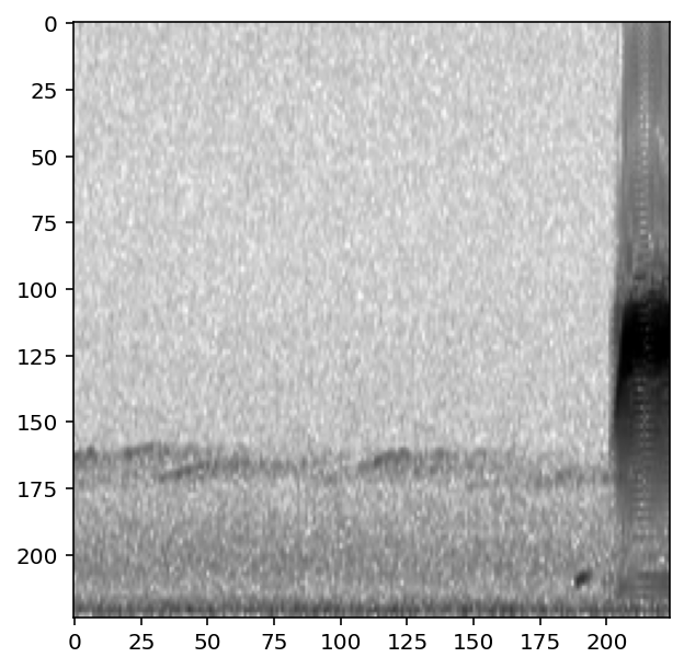
Inspect training images

Before creating a machine learning algorithm, we strongly recommend making sure the images coming out of the preprocessor look like you expect them to. Here we generate images for a few samples.

First, in order to view the images, we need a helper function that correctly displays the Tensor that comes out of the Preprocessor.

# helper function for displaying a sample as an image
def show_tensor(sample):
    plt.imshow((sample['X'][0,:,:]/2+0.5)*-1,cmap='Greys',vmin=-1,vmax=0)
    plt.show()

Now, load a handful of random samples, printing the labels and image for each:

for i, d in enumerate(train_dataset.sample(n=4)):
    print(f"labels: {d['y']}")
    show_tensor(d)

labels: tensor([0, 1])

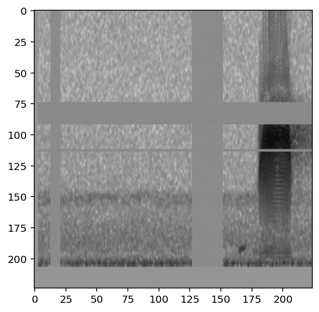
labels: tensor([1, 0])

labels: tensor([0, 1])

labels: tensor([0, 1])

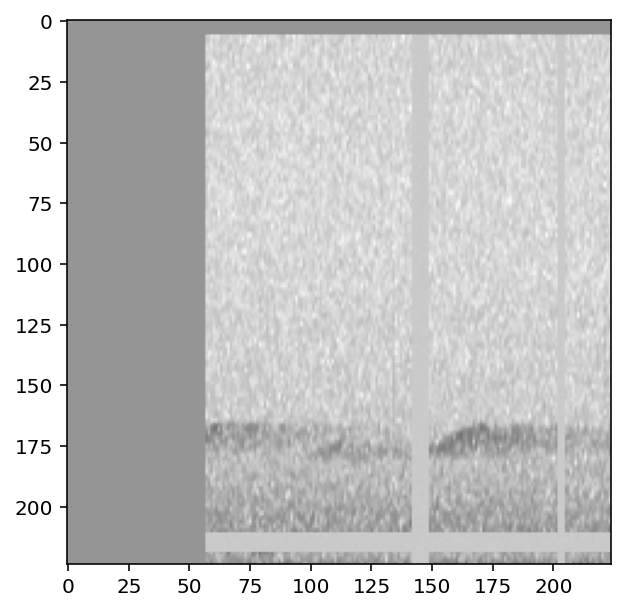
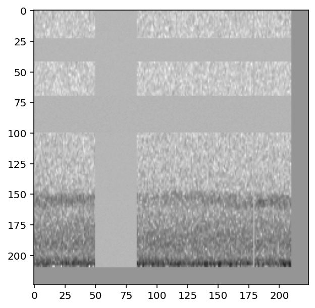
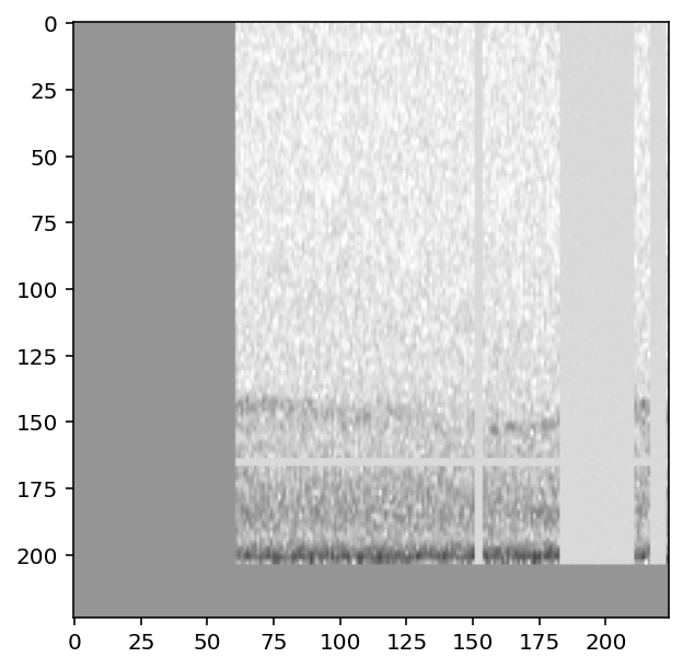
The CnnPreprocessor preprocessor allows you to turn all augmentation off or on as desired. Inspect the unaugmented images as well:

train_dataset.augmentation_off()
for i, d in enumerate(train_dataset.sample(n=4)):
    print(f"labels: {d['y']}")
    show_tensor(d)
#turn augmentation back on when we're done
train_dataset.augmentation_on()

labels: tensor([0, 1])

labels: tensor([0, 1])

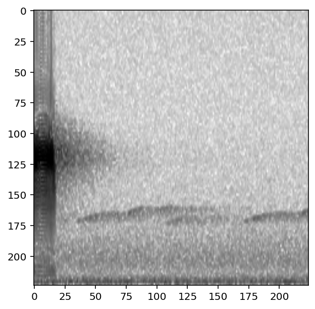
labels: tensor([1, 0])

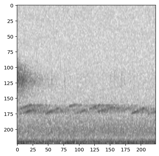
labels: tensor([0, 1])

Training

Now, we create a convolutional neural network model object, train it on the train_dataset with validation from valid_dataset, and use it for prediction.

Set up a two-class, single-target model

This demonstrates using a two class, single-target model.

• The two classes in this case are “positive” and “negative.”
• The model is “single target,” meaning that each sample belongs to exactly one class, “positive” or “negative”

We usually use two-class, single-target models to predict the presence or absence of a single species. We often refer to this as a “binary” model, but be careful not to confuse this for thresholded “binary” output predictions (1 or 0).

The model object should be initialized with a list of class names that matches the class names in the training dataset. Here we’ll use the resnet18 architecture, a popular and powerful architecture that makes a good staring point. For more details on other CNN architectures, see the “Advanced CNN Training” tutorial.

# Create model object
classes = train_df.columns
model = PytorchModel('resnet18',classes,single_target=True)

created PytorchModel model object with 2 classes

Train the model

Depending on the speed of your computer, training the CNN may take a few minutes.

We’ll only train for 5 epochs on this small dataset as a demonstration, but you’ll probably need to train for hundreds of epochs on hundreds of training files (at a minimum) to create a useful model.

In practice, using larger batch sizes (64+) improves stability and generalizability of training, particularly for architectures (such as ResNet) that contain a ‘batch norm’ layer. Here we use a small batch size to keep the computational reqirements for this tutorial low.

model.train(
    train_dataset=train_dataset,
    valid_dataset=valid_dataset,
    save_path='./binary_train/',
    epochs=5,
    batch_size=8,
    save_interval=100,
    num_workers=0,
)

Epoch: 0 [batch 0/3 (0.00%)]
        Jacc: 0.062 Hamm: 0.875 DistLoss: 1.151

Validation.
(6, 2)
         Precision: 0.4166666666666667
         Recall: 0.5
         F1: 0.45454545454545453
Updating best model
Epoch: 1 [batch 0/3 (0.00%)]
        Jacc: 0.250 Hamm: 0.500 DistLoss: 2.262

Validation.
(6, 2)
         Precision: 0.4166666666666667
         Recall: 0.5
         F1: 0.45454545454545453
Epoch: 2 [batch 0/3 (0.00%)]
        Jacc: 0.583 Hamm: 0.250 DistLoss: 0.505

Validation.
(6, 2)
         Precision: 0.4166666666666667
         Recall: 0.5
         F1: 0.45454545454545453
Epoch: 3 [batch 0/3 (0.00%)]
        Jacc: 0.375 Hamm: 0.250 DistLoss: 1.272

Validation.
(6, 2)
         Precision: 0.4166666666666667
         Recall: 0.5
         F1: 0.45454545454545453
Epoch: 4 [batch 0/3 (0.00%)]
        Jacc: 0.679 Hamm: 0.125 DistLoss: 0.374

Validation.
(6, 2)
         Precision: 0.4166666666666667
         Recall: 0.5
         F1: 0.45454545454545453
Saving weights, metrics, and train/valid scores.

Best Model Appears at Epoch 0 with F1 0.455.

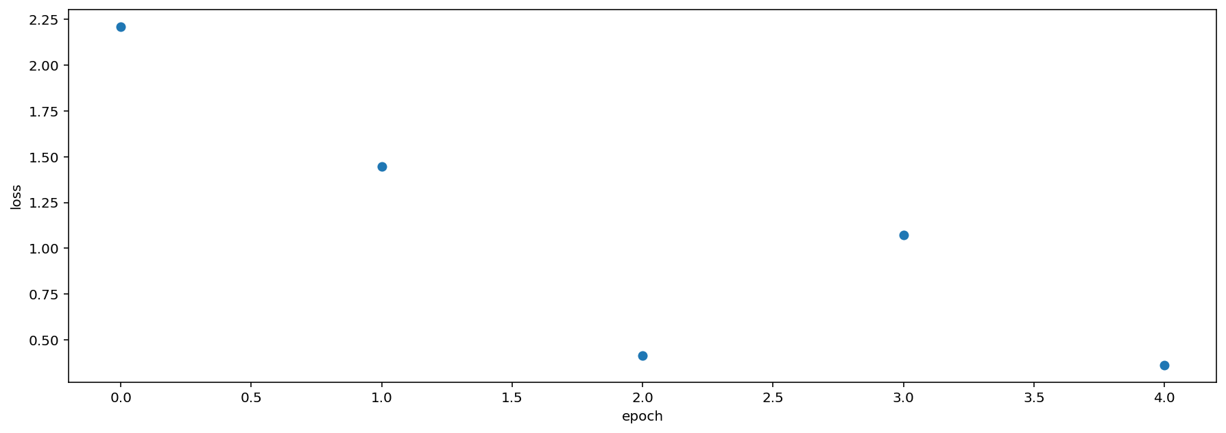
Plot the loss history

We can plot the loss from each epoch to check that our loss is declining

plt.scatter(model.loss_hist.keys(),model.loss_hist.values())
plt.xlabel('epoch')
plt.ylabel('loss')

Text(0, 0.5, 'loss')

model.save('~/Downloads/example.model')

Prediction

We haven’t actually trained a useful model in 5 epochs, but we can use the trained model to demonstrate how prediction works and show several of the settings useful for prediction.

Create preprocessor for prediction

Similar to training, prediction requires the use of a Preprocessor. To ensure that the preprocessing matches that used during model training, we’ll create our prediction Preprocessor using the training preprocessor as a starting point. (If you load a trained model from a file, you can access model.train_dataset).

In this instance, we’ll reuse the validation dataset used above, but in a real application you would likely want to use the model for prediction on a separate dataset, such as a new and unlabeled dataset that you want to classify.

#create a copy of the training dataset, sampling 0 of the training samples from it
prediction_dataset = model.train_dataset.sample(n=0)
#turn off augmentation on this dataset
prediction_dataset.augmentation_off()
#use the validation samples as test samples for the sake of illustration
prediction_dataset.df = valid_df

Predict on the validation dataset

We simply call model’s .predict() method on a Preprocessor instance.

This will return three dataframes:

• scores : numeric predictions from the model for each sample and class (by default these are raw outputs from the model)
• predictions: 0/1 predictions from the model for each sample and class (only generated if binary_predictions argument is supplied)
• labels: Original labels from the dataset, if available

valid_scores_df, valid_preds_df, valid_labels_df = model.predict(prediction_dataset)
valid_scores_df.head()

(6, 2)

	absent	present
./woodcock_labeled_data/882de25226ed989b31274eead6630b47.wav	-34.736469	34.712406
./woodcock_labeled_data/92647ab903049a9ee4125abdf7b24f2a.wav	-29.079432	28.833181
./woodcock_labeled_data/75b2f63e032dbd6d197900495a16856f.wav	-26.357983	26.485283
./woodcock_labeled_data/01c5d0c90bd4652f308fd9c73feb1bf5.wav	-35.237747	35.949291
./woodcock_labeled_data/ad14ac7ffa729060712b442e55aebf0b.wav	-6.998813	8.033541

# None: not generated because the `binary_predictions` argument was not supplied
valid_preds_df

valid_labels_df.head()

	absent	present
./woodcock_labeled_data/882de25226ed989b31274eead6630b47.wav	0	1
./woodcock_labeled_data/92647ab903049a9ee4125abdf7b24f2a.wav	0	1
./woodcock_labeled_data/75b2f63e032dbd6d197900495a16856f.wav	0	1
./woodcock_labeled_data/01c5d0c90bd4652f308fd9c73feb1bf5.wav	0	1
./woodcock_labeled_data/ad14ac7ffa729060712b442e55aebf0b.wav	1	0

The valid_preds dataframe in the example above is None - this is because we haven’t specified an option for the binary_preds argument of predict. We can choose between 'single_target' prediction (always predict the highest scoring class and no others) or 'multi_target' (predict 1 for all classes exceeding a threshold).

Create presence/absence (0/1) predictions

Supplying the binary_preds argument returns a dataframe in which the scores are transformed from continuous numbers to either 0 or 1.

Note: Binary predictions always have some error rates, sometimes large ones. It is not generally advisable to use these binary predictions as scientific observations without a thorough understanding of the model’s false-positive and false-negative rates.

If you wish to output binary predictions, three options are available:

• None: default. do not create or return binary predictions
• 'single_target': predict that the highest-scoring class = 1, all others = 0
• 'multi_target': provide a threshold. Scores above threshold = 1, others = 0

For instance, using the option 'single_target' chooses whichever of 'negative' or 'positive' is higher.

scores,preds,labels = model.predict(prediction_dataset,binary_preds='single_target')
preds.head()

(6, 2)

	absent	present
./woodcock_labeled_data/882de25226ed989b31274eead6630b47.wav	0.0	1.0
./woodcock_labeled_data/92647ab903049a9ee4125abdf7b24f2a.wav	0.0	1.0
./woodcock_labeled_data/75b2f63e032dbd6d197900495a16856f.wav	0.0	1.0
./woodcock_labeled_data/01c5d0c90bd4652f308fd9c73feb1bf5.wav	0.0	1.0
./woodcock_labeled_data/ad14ac7ffa729060712b442e55aebf0b.wav	0.0	1.0

The 'multi_target' option allows you to select a threshold. If a score meets that threshold, the binary prediction is 1; otherwise, it is 0.

Each score will have a function applied to it that takes the score from the real numbers, (-inf, inf), to the range [0, 1] (specifically the logistic sigmoid, or expit function). Whether the score meets this threshold will be based off of the sigmoid, not the raw score.

score_df, pred_df, label_df = model.predict(
    prediction_dataset,
    binary_preds='multi_target',
    threshold=0.99,
)
pred_df.head()

(6, 2)

	absent	present
./woodcock_labeled_data/882de25226ed989b31274eead6630b47.wav	0.0	1.0
./woodcock_labeled_data/92647ab903049a9ee4125abdf7b24f2a.wav	0.0	1.0
./woodcock_labeled_data/75b2f63e032dbd6d197900495a16856f.wav	0.0	1.0
./woodcock_labeled_data/01c5d0c90bd4652f308fd9c73feb1bf5.wav	0.0	1.0
./woodcock_labeled_data/ad14ac7ffa729060712b442e55aebf0b.wav	0.0	1.0

Note that in some of the above predictions, both the negative and positive classes are predicted to be present. This is because the 'multi_target' option assumes that the classes are not mutually exclusive. For a presence/absence model like the one above, the 'single_target' option is more appropriate.

Change the activation layer

We can modify the final activation layer to change the scores returned by the predict() function. Note that this does not impact the results of the binary predictions (described above), which are always calcuated using a sigmoid transformation (for multi-target models) or softmax function (for single-target models).

Options include:

• None: default. Just the raw outputs of the network, which are in (-inf, inf)
• 'softmax': scores across all classes will sum to 1 for each sample
• 'softmax_and_logit': softmax the scores across all classes so they sum to 1, then apply the “logit” transformation to these scores, taking them from [0,1] back to (-inf,inf)
• 'sigmoid': transforms each score individually to [0, 1] without requiring they sum to 1

In this case, since we are choosing between two mutually exclusive classes, we want to use the 'softmax' activation.

valid_scores, valid_preds, valid_labels = model.predict(prediction_dataset, activation_layer='softmax')

(6, 2)

Compare the softmax scores to the true labels for this dataset, side-by-side:

valid_scores.columns = ['pred_negative','pred_positive']
valid_dataset.df.join(valid_scores).sample(5)

	absent	present	pred_negative	pred_positive
filename
./woodcock_labeled_data/92647ab903049a9ee4125abdf7b24f2a.wav	0	1	7.061090e-26	1.0
./woodcock_labeled_data/ad14ac7ffa729060712b442e55aebf0b.wav	1	0	2.961637e-07	1.0
./woodcock_labeled_data/4afa902e823095e03ba23ebc398c35b7.wav	0	1	3.963297e-28	1.0
./woodcock_labeled_data/75b2f63e032dbd6d197900495a16856f.wav	0	1	1.123211e-23	1.0
./woodcock_labeled_data/01c5d0c90bd4652f308fd9c73feb1bf5.wav	0	1	1.212999e-31	1.0

Parallelizing prediction

Two parameters can be used to increase prediction efficiency, depending on the computational resources available:

• num_workers: Pytorch’s method of parallelizing across cores (CPUs) - choose 0 to predict on the root process, or >1 if you want to use more than 1 CPU
• batch_size: number of samples to predict on simultaneously

score_df, pred_df, label_df = model.predict(
    valid_dataset,
    batch_size=8,
    num_workers=0,
    binary_preds='multi_target'
)

(6, 2)

Multi-class models

A multi-class model can have any number of classes, and can be either

• multi-target: any number of classes can be positive for one sample
• single-target: exactly one class is positive for each sample

Models that are multi-target benefit from a modified loss function, and we have implemented a special class called CnnResampleLoss specifically designed for multi-target problems. We can use it similarly to the PytorchModel class:

from opensoundscape.torch.models.cnn import CnnResampleLoss
model = CnnResampleLoss('resnet18',classes)
print("model.single_target:", model.single_target)

created PytorchModel model object with 2 classes
model.single_target: False

If you want a single-target model, uncomment and run the following line.

#model.single_target = True

Train

Training looks the same as in two-class models.

model.train(
    train_dataset=train_dataset,
    valid_dataset=valid_dataset,
    save_path='./multilabel_train/',
    epochs=1,
    batch_size=16,
    save_interval=100,
    num_workers=0
)

Epoch: 0 [batch 0/2 (0.00%)]
        Jacc: 0.500 Hamm: 0.500 DistLoss: 22.018

Validation.
(6, 2)
         Precision: 0.4166666666666667
         Recall: 0.5
         F1: 0.45454545454545453
Saving weights, metrics, and train/valid scores.
Updating best model

Best Model Appears at Epoch 0 with F1 0.455.

Predict

Prediction looks the same as demonstrated above, but make sure to think carefully:

• What activation_layer do I want?
• If outputting binary predictions for each sample and class, is my model single-target (binary_preds='single_target') or multi-target (binary_preds='multi_target')?

For more detail on these choices, see the sections about activation layers and binary predictions above.

train_preds,_,_ = model.predict(train_dataset)
train_preds.columns = ['pred_negative','pred_positive']
train_dataset.df.join(train_preds).head()

(23, 2)

	absent	present	pred_negative	pred_positive
filename
./woodcock_labeled_data/49890077267b569e142440fa39b3041c.wav	0	1	-4.728383	3.845540
./woodcock_labeled_data/ad90eefb6196ca83f9cf43b6f56c4b4a.wav	0	1	-5.338425	4.401108
./woodcock_labeled_data/e9e7153d11de3ac8fc3f7164d43bac92.wav	0	1	-6.712691	5.315771
./woodcock_labeled_data/c057a4486b25cd638850fc07399385b2.wav	0	1	-4.538961	3.375217
./woodcock_labeled_data/0c453a87185d8c7ce05c5c5ac5d525dc.wav	0	1	-4.409285	3.186363

Save and load models

Models can be easily saved to a file and loaded at a later time. If the model was saved with OpenSoundscape version >=0.6.1, the entire model object will be saved - including the class, cnn architecture, loss function, and training/validation datasets. Models saved with earlier versions of OpenSoundscape do not contain all of this information and may require that you know their class and architecture (see below).

Save

OpenSoundscape saves models automatically during training:

• The model saves weights to self.save_path to epoch-X.model automatically during training every save_interval epochs
• The model keeps the file best.model updated with the weights that achieve the best F1 score on the validation dataset

You can also save the model manually at any time with model.save(path).

model1 = PytorchModel('resnet18',classes,single_target=True)
# Save every 2 epochs
model1.train(
    train_dataset=train_dataset,
    valid_dataset=valid_dataset,
    epochs=3,
    batch_size=8,
    save_path='./binary_train/',
    save_interval=2,
    num_workers=0
)
model1.save('./binary_train/my_favorite.model')

created PytorchModel model object with 2 classes
Epoch: 0 [batch 0/3 (0.00%)]
        Jacc: 0.314 Hamm: 0.500 DistLoss: 0.727

Validation.
(6, 2)
         Precision: 0.4166666666666667
         Recall: 0.5
         F1: 0.45454545454545453
Updating best model
Epoch: 1 [batch 0/3 (0.00%)]
        Jacc: 0.250 Hamm: 0.500 DistLoss: 1.237

Validation.
(6, 2)
         Precision: 0.4166666666666667
         Recall: 0.5
         F1: 0.45454545454545453
Saving weights, metrics, and train/valid scores.
Epoch: 2 [batch 0/3 (0.00%)]
        Jacc: 0.375 Hamm: 0.250 DistLoss: 0.549

Validation.
(6, 2)
         Precision: 0.4166666666666667
         Recall: 0.5
         F1: 0.45454545454545453
Saving weights, metrics, and train/valid scores.

Best Model Appears at Epoch 0 with F1 0.455.

Load

Models created with OpenSoundscape 0.6.1 and above can be loaded in their entirety with the load_model function:

from opensoundscape.torch.models.cnn import load_model
model = load_model('./binary_train/best.model')

The model can now be used for prediction (model.predict()) or to continue training (model.train()).

Predict using saved model

Using a saved or downloaded model to run predictions on audio files is as simple as

1. Loading a previously svaed model
2. Creating an instance of a preprocessor class for prediction
3. Running model.predict() on the preprocessor

# load the saved model
model = load_model('./binary_train/best.model')

# create a Preprocessor instance with the audio samples
# use the model.train_dataset as a starting point to ensure that our preprocessing matches what the model expects
prediction_dataset = model.train_dataset.sample(n=0)
prediction_dataset.augmentation_off()
prediction_dataset.df = valid_df

#predict on a dataset
scores,_,_ = model.predict(prediction_dataset, activation_layer='softmax_and_logit')

(6, 2)

Continue training from saved model

Similar to predicting using a saved model, we can also continue to train a model after loading it from a saved file.

By default, .load() loads the optimizer parameters and learning rate parameters from the saved model, in addition to the network weights.

# Create architecture
model = load_model('./binary_train/best.model')

# Continue training from the checkpoint where the model was saved
model.train(train_dataset,valid_dataset,save_path='.',epochs=0)

Best Model Appears at Epoch 0 with F1 0.000.

Next steps

You now have seen the basic usage of training CNNs with OpenSoundscape and generating predictions.

Additional tutorials you might be interested in are: * Custom preprocessing: how to change spectrogram parameters, modify augmentation routines, etc. * Custom training: how to modify and customize model training * Predict with pre-trained CNNs: details on how to predict with pre-trained CNNs. Much of this information was covered in the tutorial above, but this tutorial also includes information about using models made with previous versions of OpenSoundscape

Finally, clean up and remove files created during this tutorial:

import shutil
dirs = ['./multilabel_train', './binary_train', './woodcock_labeled_data']
[shutil.rmtree(d) for d in dirs]

[None, None, None]