Use a CNN to recognize sounds

This notebook contains all the code you need to use an existing (pre-trained) OpenSoundscape convolutional neural network model (CNN) to make predictions on your own data - for instance, to detect the song or call of an animal the CNN has been trained to recognize. It asssumes that you already have access to a CNN that has been trained to recognize the sound of interest.

To find publicly available pre-trained CNNs, check out the Bioacoustics Model Zoo.

If you are interested in training your own CNN, see the other tutorials at opensoundscape.org related to model training.

Before running this tutorial, install OpenSoundscape by following the instructions on the OpenSoundscape website, opensoundscape.org. More detailed tutorials about data preprocessing, training CNNs, and customizing prediction methods can also be found on this site.

Run this tutorial

This tutorial is more than a reference! It’s a Jupyter Notebook which you can run and modify on Google Colab or your own computer.

Link to tutorial	How to run tutorial
	The link opens the tutorial in Google Colab. Uncomment the “installation” line in the first cell to install OpenSoundscape.
	The link downloads the tutorial file to your computer. Follow the Jupyter installation instructions, then open the tutorial file in Jupyter.

# if this is a Google Colab notebook, install opensoundscape in the runtime environment
if 'google.colab' in str(get_ipython()):
  %pip install "opensoundscape==0.13.0" "jupyter-client<8,>=5.3.4" "ipykernel==6.17.1"

package imports

The cnn module provides a function load_model to load saved opensoundscape models

from opensoundscape.ml.cnn import load_model
from opensoundscape import Audio
import opensoundscape

load some additional packages and perform some setup for the Jupyter notebook.

# Other utilities and packages
import torch
from pathlib import Path
import numpy as np
import pandas as pd
from glob import glob
import subprocess

#set up plotting
from matplotlib import pyplot as plt
plt.rcParams['figure.figsize']=[15,5] #for large visuals
%config InlineBackend.figure_format = 'retina'

Load a model

Models can be loaded either from a local file (load_model(file_path)) or directly from the Bioacoustics Model Zoo like this:

Note: make sure to install the bioacoustics_model_zoo as a package in your python environment:

pip install bioacoustics-model-zoo==0.12.0

After installing, a running notebook must be restarted to gain access to the package

import bioacoustics_model_zoo as bmz

# list available models from the model zoo
bmz.utils.list_models()

{'BirdNET': bioacoustics_model_zoo.birdnet.BirdNET,
 'BirdNETOccurrenceModel': bioacoustics_model_zoo.birdnet.BirdNETOccurrenceModel,
 'Perch2LiteRT': bioacoustics_model_zoo.perch_v2_litert.Perch2LiteRT,
 'SeparationModel': bioacoustics_model_zoo.mixit_separation.SeparationModel,
 'YAMNet': bioacoustics_model_zoo.yamnet.YAMNet,
 'Perch': bioacoustics_model_zoo.perch.Perch,
 'Perch2': bioacoustics_model_zoo.perch_v2.Perch2,
 'HawkEars': bioacoustics_model_zoo.hawkears.hawkears.HawkEars,
 'HawkEars_Low_Band': bioacoustics_model_zoo.hawkears.hawkears.HawkEars_Low_Band,
 'HawkEars_Embedding': bioacoustics_model_zoo.hawkears.hawkears.HawkEars_Embedding,
 'HawkEars_v010': bioacoustics_model_zoo.hawkears.hawkears.HawkEars_v010,
 'BirdSetConvNeXT': bioacoustics_model_zoo.bmz_birdset.bmz_birdset_convnext.BirdSetConvNeXT,
 'BirdSetEfficientNetB1': bioacoustics_model_zoo.bmz_birdset.bmz_birdset_efficientnetB1.BirdSetEfficientNetB1,
 'RanaSierraeCNN': bioacoustics_model_zoo.rana_sierrae_cnn.RanaSierraeCNN}

Some models require additional dependencies. HawkEars requires the timm and torchaudio packages to be installed in your environment.

hawkears = bmz.HawkEars()

Choose audio files for prediction

Create a list of audio files to predict on. They can be of any length. Consider using glob to find many files at once.

For this example, let’s download a 1-minute audio clip:

url = "https://tinyurl.com/birds60s"
Audio.from_url(url).save("./1min.wav")

use glob to create a list of all files matching a pattern in a folder:

from glob import glob

audio_files = glob("./*.wav")  # match all .wav files in the current directory
audio_files

['./demo_audio.wav', './1min.wav']

Listening to the recording, we can hear songs and calls of Wood Thrush, Ovenbird, Black-and-white Warblers, Hooded Warblers, and more.

Audio.from_file(audio_files[0])

generate predictions with the model

The model returns a dataframe with a MultiIndex of file, start_time, and end_time. There is one column for each class.

The values returned by the model range from -infinity to infinity (theoretically), and higher scores mean the model is more confident the class (song/species/sound type) is present in the audio clip.

scores = hawkears.predict(audio_files)
scores.head()

			American Bullfrog	American Toad	Boreal Chorus Frog	Canine	Canadian Toad	Gray Treefrog	Great Plains Toad	Green Frog	Northern Leopard Frog	Mashup	...	Yellow Rail	Yellow Warbler	Yellow-bellied Flycatcher	Yellow-bellied Sapsucker	Yellow-billed Cuckoo	Yellow-breasted Chat	Yellow-headed Blackbird	Yellow-rumped Warbler	Yellow-throated Vireo	Yellow-throated Warbler
file	start_time	end_time
./demo_audio.wav	0.0	3.0	-3.466256	-3.448090	-3.493556	-3.503592	-3.481331	-3.487176	-3.483800	-3.437101	-3.500467	-3.496845	...	-3.476843	-3.523676	-3.492661	-3.503134	-3.464896	-3.496201	-3.435257	-3.562006	-3.346351	-3.482978
	3.0	6.0	-3.457553	-3.479793	-3.474909	-3.500456	-3.487077	-3.522441	-3.459663	-3.442261	-3.505857	-3.440974	...	-3.526970	-3.626572	-3.534512	-3.563111	-3.492841	-3.466604	-3.528344	-3.432244	-3.378526	-3.413256
	6.0	9.0	-3.474403	-3.448281	-3.479034	-3.503640	-3.475060	-3.477652	-3.478258	-3.470358	-3.468938	-3.492811	...	-3.464751	-3.474232	-3.492598	-3.465265	-3.438451	-3.503668	-3.502397	-3.518036	-3.554748	-3.507980
	9.0	12.0	-3.462986	-3.505934	-3.457190	-3.485591	-3.492722	-3.488315	-3.466021	-3.464118	-3.502368	-3.466348	...	-3.493623	-3.363047	-3.474586	-3.527257	-3.504027	-3.485874	-3.472647	-3.593486	-3.486274	-3.522454
	12.0	15.0	-3.470327	-3.487154	-3.470491	-3.424055	-3.488506	-3.491496	-3.468609	-3.442134	-3.455426	-3.453564	...	-3.494715	-3.489774	-3.448597	-3.446382	-3.451458	-3.462630	-3.458184	-3.473811	-3.375827	-3.494082

5 rows × 353 columns

We might want overlapping prediction time windows, to ensure sounds are not missed because they are cut off on the edge of a clip

We’ll also use ‘batch size’ to increase the number of samples predicted on at a time. When GPU is available for accelerating inference, large batch sizes like 64, 128, or 512 greatly speed up inference. Use as large of a batch size as you can without getting a CUDA out of memory error.

scores = hawkears.predict(audio_files, overlap_fraction=0, batch_size=8)
scores.head()

			American Bullfrog	American Toad	Boreal Chorus Frog	Canine	Canadian Toad	Gray Treefrog	Great Plains Toad	Green Frog	Northern Leopard Frog	Mashup	...	Yellow Rail	Yellow Warbler	Yellow-bellied Flycatcher	Yellow-bellied Sapsucker	Yellow-billed Cuckoo	Yellow-breasted Chat	Yellow-headed Blackbird	Yellow-rumped Warbler	Yellow-throated Vireo	Yellow-throated Warbler
file	start_time	end_time
./demo_audio.wav	0.0	3.0	-3.466256	-3.448090	-3.493556	-3.503592	-3.481331	-3.487176	-3.483800	-3.437101	-3.500467	-3.496845	...	-3.476843	-3.523676	-3.492661	-3.503134	-3.464896	-3.496201	-3.435257	-3.562006	-3.346351	-3.482978
	3.0	6.0	-3.457553	-3.479793	-3.474909	-3.500456	-3.487077	-3.522441	-3.459663	-3.442261	-3.505857	-3.440974	...	-3.526970	-3.626572	-3.534512	-3.563111	-3.492841	-3.466604	-3.528344	-3.432244	-3.378526	-3.413256
	6.0	9.0	-3.474403	-3.448280	-3.479034	-3.503640	-3.475060	-3.477652	-3.478258	-3.470358	-3.468938	-3.492811	...	-3.464751	-3.474232	-3.492598	-3.465265	-3.438450	-3.503668	-3.502397	-3.518036	-3.554748	-3.507980
	9.0	12.0	-3.462986	-3.505934	-3.457190	-3.485591	-3.492722	-3.488315	-3.466021	-3.464118	-3.502368	-3.466348	...	-3.493623	-3.363047	-3.474586	-3.527257	-3.504027	-3.485874	-3.472647	-3.593486	-3.486274	-3.522454
	12.0	15.0	-3.470327	-3.487154	-3.470491	-3.424055	-3.488506	-3.491496	-3.468609	-3.442134	-3.455426	-3.453564	...	-3.494715	-3.489774	-3.448597	-3.446382	-3.451458	-3.462630	-3.458184	-3.473811	-3.375827	-3.494082

5 rows × 353 columns

adding an activation function

The code above returns the raw predictions of the model without any post-processing (such as a softmax layer or a sigmoid layer).

For details on how to post-processing prediction scores and to generate binary 0/1 predictions of class presence, see the “Basic training and prediction with CNNs” tutorial notebook. But, as a quick example here, let’s add a softmax layer to make the prediction scores for both classes sum to 1.

We can also convert our continuous scores into True/False (or 1/0) predictions for the presence of each class in each sample. Think about whether each clip should be labeled with only one class or whether each clip could contain zero, one, or multiple classes

We can map the raw “logit” outputs from the CNN onto the range 0-1 by applying the sigmoid activation function, which is appropriate for multi-target classification

scores = hawkears.predict(audio_files, activation_layer="sigmoid", overlap_fraction=0.5)
scores.head()

			American Bullfrog	American Toad	Boreal Chorus Frog	Canine	Canadian Toad	Gray Treefrog	Great Plains Toad	Green Frog	Northern Leopard Frog	Mashup	...	Yellow Rail	Yellow Warbler	Yellow-bellied Flycatcher	Yellow-bellied Sapsucker	Yellow-billed Cuckoo	Yellow-breasted Chat	Yellow-headed Blackbird	Yellow-rumped Warbler	Yellow-throated Vireo	Yellow-throated Warbler
file	start_time	end_time
./demo_audio.wav	0.0	3.0	0.030288	0.030826	0.029496	0.029210	0.029848	0.029679	0.029777	0.031156	0.029299	0.029402	...	0.029978	0.028646	0.029522	0.029223	0.030328	0.029421	0.031212	0.027599	0.034015	0.029800
	1.5	4.5	0.029713	0.030142	0.029928	0.029630	0.030406	0.029130	0.029963	0.030580	0.031033	0.029469	...	0.029939	0.029363	0.030038	0.031194	0.029792	0.029825	0.029604	0.029126	0.036767	0.036750
	3.0	6.0	0.030544	0.029893	0.030035	0.029299	0.029682	0.028680	0.030482	0.031000	0.029146	0.031039	...	0.028555	0.025918	0.028346	0.027569	0.029517	0.030278	0.028516	0.031303	0.032973	0.031884
	4.5	7.5	0.029931	0.030016	0.029884	0.030138	0.029475	0.029137	0.030188	0.030910	0.029192	0.030261	...	0.028285	0.027128	0.028775	0.029440	0.029397	0.029045	0.029455	0.029573	0.028503	0.030980
	6.0	9.0	0.030049	0.030820	0.029915	0.029209	0.030030	0.029955	0.029937	0.030168	0.030209	0.029517	...	0.030332	0.030054	0.029524	0.030317	0.031115	0.029208	0.029244	0.028803	0.027794	0.029086

5 rows × 353 columns

Now let’s use the predict_multi_target_labels(scores) function to apply a threshold score and generate detection/non-detections.

from opensoundscape.metrics import predict_multi_target_labels

predicted_labels = predict_multi_target_labels(scores, threshold=0.7)

# count the number of detections for each species
detection_counts = predicted_labels.sum(0)
detection_counts[detection_counts > 0]

American Redstart          12
Black-and-white Warbler     4
Hooded Warbler             18
Ovenbird                    2
Wood Thrush                20
dtype: int64

Do you agree with the HawkEars detections? Do you hear any other species?

Audio.from_file(audio_files[0])

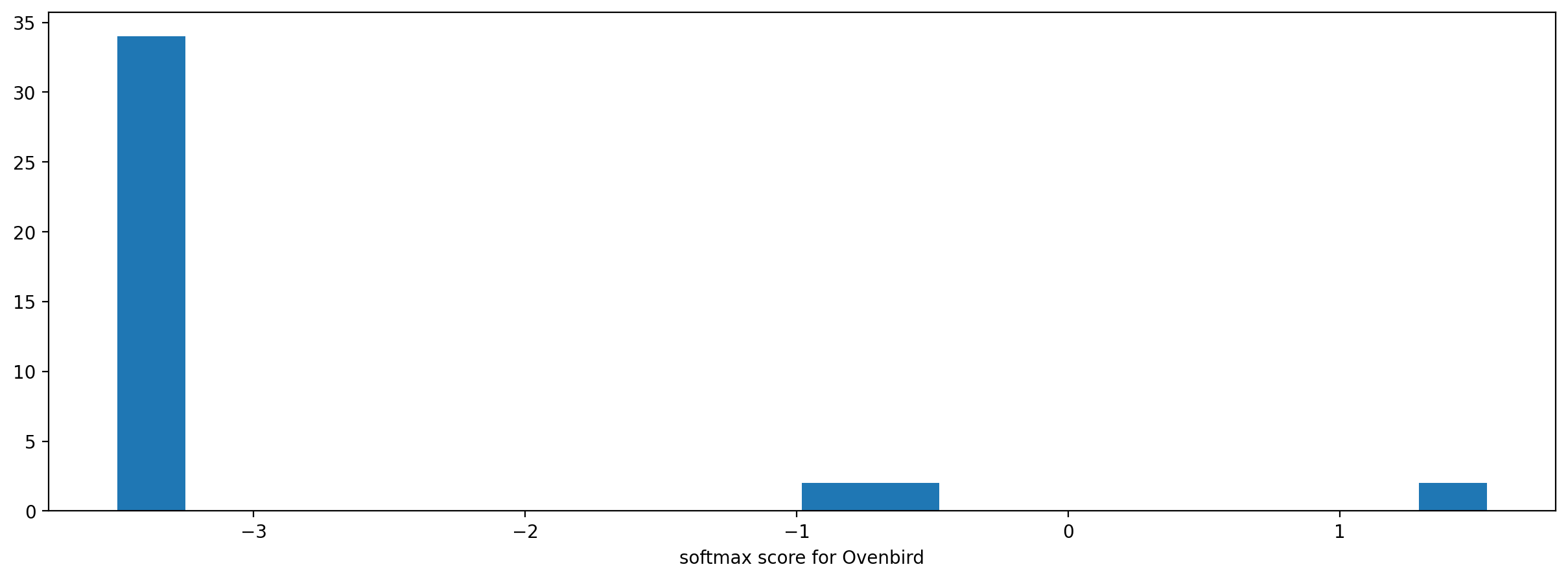
It is sometimes helpful to look at a histogram of the scores, although we only have a handful of clips here so the histogram is sparse.

_ = plt.hist(scores["Ovenbird"], bins=20)
_ = plt.xlabel("softmax score for Ovenbird")

generate embeddings with the model

Embeddings are typically the outputs of the penultimate layer of the machine learning model. The embeddings can be useful for extracting a “feature vector” for each audio sample, with various downstream applications such as recognition of new classes or clustering based on acoustic qualities. OpenSoundscape and Biaocoustic Model Zoo classification models have a .embed() method with similar inputs and outputs to the .predict() method. Each row in the output is the embedding vector for one audio clip.

embeddings = hawkears.embed(audio_files)
embeddings.head()

			0	1	2	3	4	5	6	7	8	9	...	1910	1911	1912	1913	1914	1915	1916	1917	1918	1919
file	start_time	end_time
./demo_audio.wav	0.0	3.0	0.000000	0.000000	0.0	0.005686	0.0	0.000000	0.0	0.0	0.0	0.001031	...	0.009462	0.0	0.000000	0.0	0.003263	0.000000	0.000000	0.000550	0.000335	0.00000
	3.0	6.0	0.000000	0.014767	0.0	0.000000	0.0	0.002209	0.0	0.0	0.0	0.000000	...	0.000000	0.0	0.000415	0.0	0.000000	0.011083	0.001684	0.005371	0.000000	0.00000
	6.0	9.0	0.005847	0.000000	0.0	0.000000	0.0	0.000348	0.0	0.0	0.0	0.003157	...	0.017381	0.0	0.000000	0.0	0.000104	0.000000	0.000000	0.000000	0.000000	0.00000
	9.0	12.0	0.033705	0.023867	0.0	0.002927	0.0	0.000000	0.0	0.0	0.0	0.003928	...	0.003397	0.0	0.000000	0.0	0.007739	0.000000	0.000000	0.009266	0.000000	0.00115
	12.0	15.0	0.000000	0.013020	0.0	0.001521	0.0	0.000000	0.0	0.0	0.0	0.007852	...	0.000000	0.0	0.000000	0.0	0.000000	0.000000	0.000000	0.002100	0.000000	0.00000

5 rows × 1920 columns

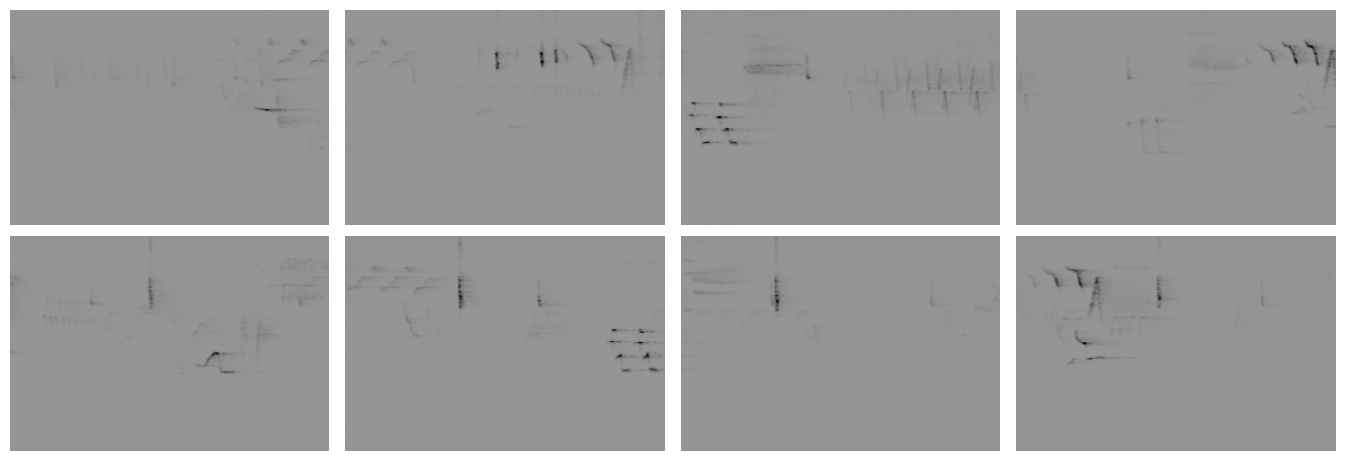
Inspect samples generated during prediction

from opensoundscape.preprocess.utils import show_tensor_grid
from opensoundscape.ml.datasets import AudioFileDataset

# generate a dataset with the samples we wish to generate and the model's preprocessor
inspection_dataset = AudioFileDataset(audio_files, hawkears.preprocessor)
inspection_dataset.bypass_augmentations = True

# Note: hawkears produces samples "upside down" relative to the usual convention (low frequencies at bottom of image)
# so we flip the samples for visualization here
samples = [sample.data.flip(1) for sample in inspection_dataset.head(8)]
_ = show_tensor_grid(samples, 4)

Activation maps: understand what the model is looking at

GradCAM (gradient-class activation maps) is a tool for visualizing which parts of a sample caused the CNN to predict a specific class was present. This is a great way to check that the model is paying attention to the right things, or understand why the model makes certain types of mistakes. We’ve built in GradCAM into the opensoundscape CNN class so that its easy to apply

Let’s take the Ovenbird and Wood Thrush in the 3rd sample as an example, and ask the model which parts of the sample made it confident that Ovenbird was present

We specify guided_backprop=True here: without this option, CAMs are generated for general regions of the image, but with this option we get pixel-level activations from the input.

By using the “backprop and activation” mode, we visualize the combination of (a) the general region of activation on the final layer with (b) the specific pixels from the input.

Audio.from_file(audio_files[0], offset=6, duration=3)

# define the audio segments we wish to generate CAMs for
samples_df = pd.DataFrame(
    {"file": audio_files[0:1], "start_time": [6], "end_time": [9]}
).set_index(["file", "start_time", "end_time"])

# generate CAMs for Ovenbird class with guided backpropagation
# noe: requires optional dependency `pip install grad-cam``
samples_with_cams = hawkears.generate_cams(
    samples_df, classes=["Ovenbird", "Wood Thrush"], guided_backprop=True
)

# plot the CAM for the Ovenbird class for the 3rd sample
samples_with_cams[0].cam.plot(mode="backprop_and_activation", flipud=True)

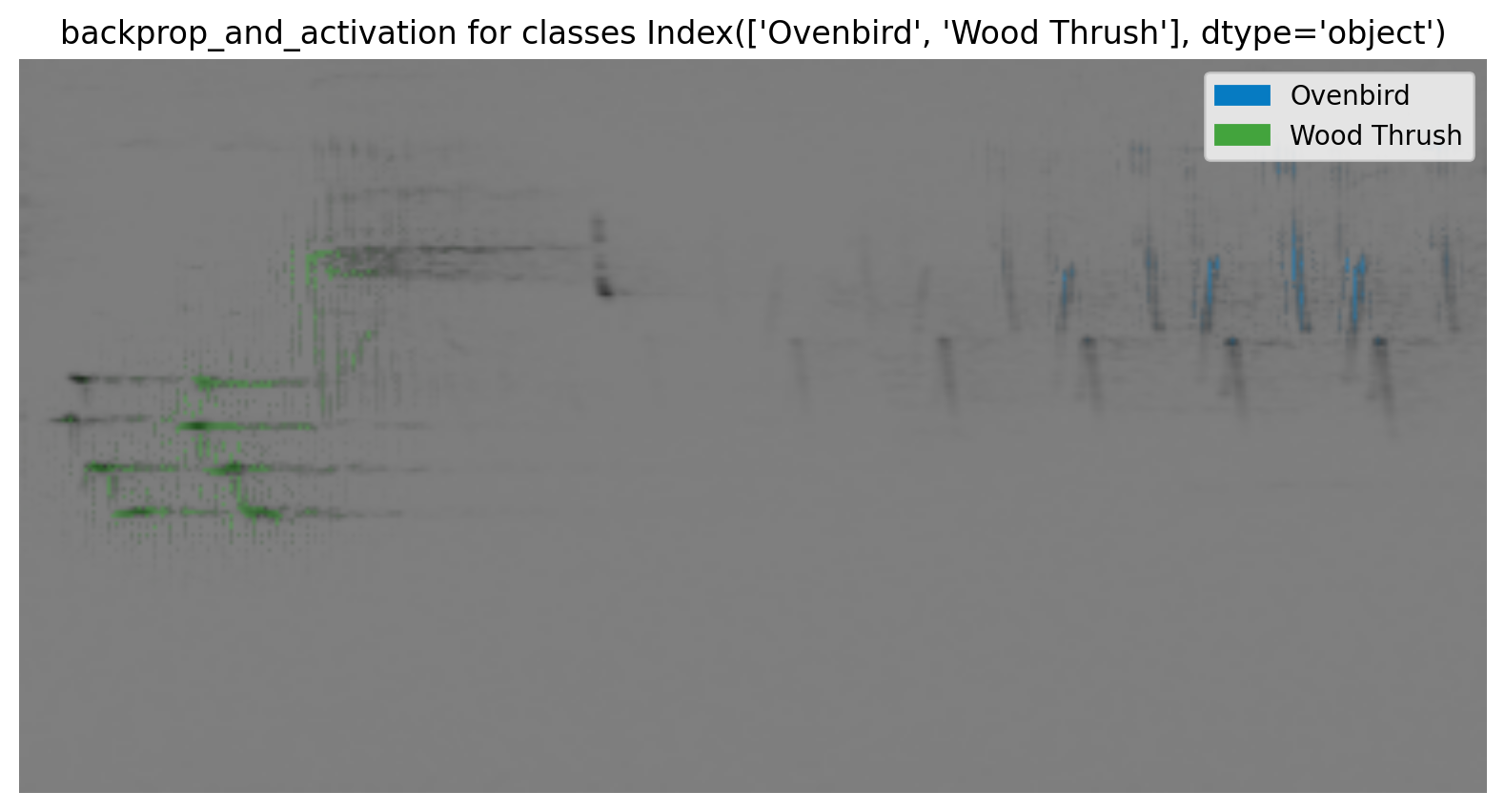
(<Figure size 1500x500 with 1 Axes>,
 <Axes: title={'center': "backprop_and_activation for classes Index(['Ovenbird', 'Wood Thrush'], dtype='object')"}>)

To dig further into the options for generating and plotting gradient activation maps, see the docstrings of CNN.generate_cams() and opensoundscape.ml.cam.CAM.plot()

Using models trained in older OpenSoundscape versions

Simply load the model with opensoundscape.ml.cnn.load_model(path).

Starting with OpenSoundscape 0.11.0, the default model.save() (for CNN/SpectroramClassifier) is designed to work smoothly across package version updates: the default behavior (pickle=False) saves a state dictionary for the network parameters and a dictionary describing the preprocessing settings, as well as some other information (class list, architecture name, etc) which OpenSoundscape can use to re-create the model from the saved file so long as any custom code used to create the model/preprocessor is still available when loading the model from a file.

In general, if you want to use a model created in an OpenSoundscape <0.11.0 in a newer version, you should:

1. use or re-create a separate Python environment (eg, conda environment) that has the same version of OpenSoundscape used to create and train the model.

2. Save the model’s weights like this:

torch.save({'weights':model.network.state_dict()},'my_weights.pt')

3. You’ll also want to save/take note of the architecture, ordered list of model classes, and sample input shape, and all preprocessing parameters/steps (e.g. sample shape, spectrogram creation parameters, scaling/normalization).

4. Then, in your new opensoundscape environment, recreate the model with the same architecture, input shape, class list, and preprocessing parameters

5. Load the saved weights into the model architecture:

weights = torch.load('my_weights.pt')['weights']
my_new_model.network.load_state_dict(weights)

Be aware of changes to default preprocessing settings between OpenSoundscape versions. In particular:

• opensoundscape<0.7.0 used the opposite sign convention in preprocessed tensor samples: loud sounds were low values and quiet sounds were high values. Specify model.preprocessor.pipeline.to_tensor.set(invert=True) to match the default preprocessor behavior of opensoundscape<0.7.0

• opensoundscape<0.11.0 used skimage interpolation by default in Spectrogram.to_tensor(which is used in the SpectrogramPreprocessor.pipeline.to_tensor action), while newer version use pytorch interpolation by default (much faster). The differences in interpolation methods are subtle but lead to slightly different ML model scores. Specify model.preprocessor.pipeline.to_tensor.set(use_skimage=True) to match the default preprocessor behavior of opensoundscape<0.11.0.

• opensoundscape<0.12.0 CNN class’s default Overlay preprocessor had update_labels=False, >=0.12.0 has default update_labels=True

If you need assistance loading a model developed in a different OpenSoundscape version into a more recent version, please contact one of the developers of OpenSoundscape.

Clean up: delete model objects

from pathlib import Path

for p in Path(".").glob("*.model"):
    p.unlink()

# uncomment to delete the downloaded audio file
# Path('1min.wav').unlink()